Additional Material for Chapter 2
Additional Material for Section 2.1
Construction of a ugraph
This "construction" will start with all the collection of nodes in a ugraph. Then it will proceed by adding edges to it from some list of edges. This may be done in a drawing if the ugraph is not to big and complicated. But it could be done by computation. If the ugraph is small then the work can be done by hand, as shown below. Otherwise the computer could do the work according to some program.
Addition of edges provides the action. Attention is focused on the components. There are two possibilities.
(A) The edge being added has end points in different components. The edge becomes a "bridge" between those components so they are no longer separate components. They become one bigger component. The number of components decreases by one.
 (B) The edge being added has end points in the same component. Then is no change in the components. However, this happens only if the added edge completes a loop. This loop will not disappear from the addition of more edges. So it will appear in the final ugraph, after all the edges in the list have been added.
Return to Chapter01
/
section 2.1
===============
Additional Material for Section 2.2
filler
filler
filler
zzzzzzzzzzzzzzzzzzzzzzzz
In Chapters 1 and 2 discussions of ugraphs dominated. But often motion is associated with trees, as used in section 2.3 of chapter 2. In this section of additional material the concept of a tree will be described as a special DIgraph. This approach is compatible with the common definition of a tree as a ugraph given in Chapter 2 and in most textbooks on graph theory.
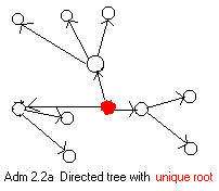
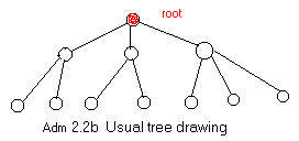
 Characteristic of a directed tree is the fact that every node is the head of exactly one arc (every node has exactly one arrow pointing to it), with one exception. The root node, or simply root, is distinguished by the fact that it is not the head of any arc (no arrow points to it). Although is customary to draw the usual undirected tree upside down with the root at the top (figure Adm 2.2b), the directed tree can unambiguously appear in any position (figure Adm 2.2a).
The leaves of a tree are nodes which are not the tail of any arcs (there are no arrows pointing away from them).
The facts that only one arrow points to each node (except for the root) and the tree is connected prevent any loops in a directed tree. At the end of any loop two arrows would point to the same node. The tree cannot be a loop because there must be a root which has no arrow pointing to it.
 In most text books on graph theory a tree is drawn as a ugraph. Arcs in figure Adm 2.2a have been repositioned to get an equivalent graph and replaced by downward sloping edges under them (the arrows are replaced by undirected line segments). The undirected tree with edges is the most common and convenient way of drawing a tree.
Replacing the arcs of a directed tree by edges produces the underlying ugraph, called the underlying or undirected tree.
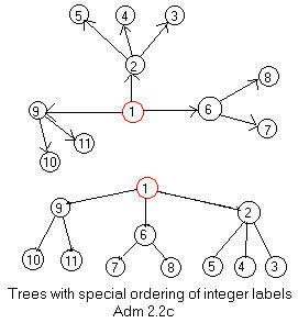 The nodes of a digraph can be assigned integer labels in many ways. Although it is not necessary, but it may be interesting that the integers can be assigned to the nodes of a directed tree in a special way. The tail of each arc has an integer less than the integer given to the head. In the undirected tree assign larger integers to lower nodes. Assign the lowest integer to the root. Going down any path assign increasing integers until a leaf is reached. Then back up and go down a different path, assigning larger and larger integers. See figure Adm 2.2c.
Now look at the two graphs in Adm 2.2c as a digraph and a ugraph. The exist adjacency arrays for them. However the arrays are identical, namely,
1,2,6,9, 2,3,4,5, 3, 4, 5, 6,7,8, 7, 8, 9,10,11, 10, 11, 0,0
The short form of the adjacency array is used for the lower ugraph (tree).
====================
Reconstructing a ugraph from a list of edges
 In section 2.2 of the main text edges were removed to get a spanning tree.
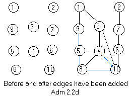
Just the reverse of removing edges is the construction of the ugraph given the nodes as a discrete collection and a list of edges to be attached to them. See figure Adm 2.2d. Edges that cause loops to be formed can be omitted. (Also omit duplicate edges if there are any.) In the construction of the ugraph here every edge that cause loops can be attached to nodes, but such edges can be given a special color, say blue. Other edges are black. Then the whole ugraph is constructed, and the spanning tree is that part of the ugraph with black edges. Therefore the tree is easily created by deleting all the blue edges.
In section 2.2 of the main text edges were removed to get a spanning tree.
Just the reverse of removing edges is the construction of the ugraph given the nodes as a discrete collection and a list of edges to be attached to them. See figure Adm 2.2d. Edges that cause loops to be formed can be omitted. (Also omit duplicate edges if there are any.) In the construction of the ugraph here every edge that cause loops can be attached to nodes, but such edges can be given a special color, say blue. Other edges are black. Then the whole ugraph is constructed, and the spanning tree is that part of the ugraph with black edges. Therefore the tree is easily created by deleting all the blue edges.
Before edges are attached, the discrete set of nodes form ten components (pieces). After all of the edges have been added in figure Adm 2.2d, there is only one component, because the ugraph is connected (the ugraph is in one piece.) However, if edge 6-10 is omitted from the list (#) of edges to be added, then there will be two components in the entire ugraph.
The list of edges to be added to the discrete set of nodes in figure Adm 2.2d is
(#) 1-3 1-9 2-7 3-4 3-10 4-5 4-8 4-10 5-8 5-9 6-7 6-10 8-10 0-0
The list of edges is in the order wher the first end point of an edge is never less than the first end point of the next edge. The right end point of every edge is greater than the left end point. To be safe always get thiss list from the short form of the adjacency list for the finished ugraph.
It is not obvious from the collection of discrete nodes together with the list (#) of edges what the components of the ugraph are, the complete picture of what pairs of nodes are connected somehow. The process to be discussed now will show what nodes are connected (by being in the same component), and at the same time show that the edges
4-10 5-8 5-9 8-10 during construction cause loops.
Each component well have its own unique label which will be called here a component marker or simply marker. All the markers will be different, so that there will be as many markers as components.
Start with the discrete collection of nodes. Then each node is a component of one node and no edges. Assign to each of these very tiny components amarker equal to the node integer label.
node 1 2 3 4 5 6 7 8 9 10
marker 1 2 3 4 5 6 7 8 9 10
As edges are added to the nodes the markers mayl change but the integer labels will always stay the same. Through the process the red color of the component markers will distinguish them from the black integer labels on the nodes.
The basic rule If an edge X-Y is to be added, then locate the markers under X and under Y. If they are different, replace the larger marker by the smaller. If they are the same, then the addition of X-Y will create a loop. In these notes X-Y becomes blue in the list (#) on the screen. On paper a symbol * (asterisk) can be written immediately after X-Y. In processing the list (#) four edges will be found to produce loops. See (####) below.
The reader is encouraged to copy the collection of the discrete nodes in figure Adm 2.2d, and add each edge to that collection at the time the edge is discussed below.
The first edge to be added is 1-3. This can be seen as dark black integers in
node 1 2 3 4 5 6 7 8 9 10
marker 1 2 1 4 5 6 7 8 9 10
The marker under the 3 has been replaced by the smaller marker under the 1.
The next edge to be added is 1-9. Replace the marker under the 9 by the marker under the 1.
node 1 2 3 4 5 6 7 8 9 10
marker 1 2 1 4 5 6 7 8 1 10
Under the three nodes 1,3,9 is the same number 1. This means that 1,3,9 along with the added edges form a component with marker 1.
The fourth basic idea: - all node integers over the same marker form a component with that marker.
After adding the edge 2-7 the table becomes
node 1 2 3 4 5 6 7 8 9 10
marker 1 2 1 4 5 6 2 8 1 10
There are now two new components: a component 1,3,9 with marker 1 and a component 2,7 with marker 2.
Add edge 3-4 to get
node 1 2 3 4 5 6 7 8 9 10
marker 1 2 1 1 5 6 2 8 1 10
Add edges 3-10, 4-5, 4-8 to get three components with markers 1,2,6:
node 1 2 3 4 5 6 7 8 9 10
marker 1 2 1 1 1 6 2 1 1 1
The addition of edge 4-10 has no effect on the markers because the markers under 4 and 10 are the same The end points 4,10 are already in component with marker 1. Therefore the addition of 4-10 creates a loop in that component.
Similarly, the addition of edges 5-8 and 5-9 make no changes in the markers because nodes 5,8,9 are already in component with marker 1. So the edges are written 5-8 and 5-9
The addition of edge 6-7 produces the table:
(##)node 1 2 3 4 5 6 7 8 9 10
(##)marker 1 2 1 1 1 1 2 1 1 1
The addition of 6-10 produces the table:
(###) node 1 2 3 4 5 6 7 8 9 10
(###)marker 1 1 1 1 1 1 1 1 1 1
The addition of 8-10 produces no effect on the array of markers in the table (###). The edge upon addition creates a loop.
Collecting the blue edges that created loops the list (#) becomes:
(####) 1-3 1-9 2-7 3-4 3-10 4-5 4-8 4-10 5-8 5-9 6-7 6-10 8-10 0-0 0-0 There are at least four loops in the finished ugraph.
This last table (###) reflects the addition of all the edges listed in (#) to the discrete nodes. All nodes in the ugraph are in component 1. The entire ugraph is equal to component 1. Therefore the ugraph is connected.
As each edge is added to the nodes, the size of one of the components increases by one new node, while the number of components decreases by one, unless that edge causes a loop to be formed. Intuitively speaking, the nodes in that component are already connected without the help of the new edge, because both of the end points of the edge already are nodes in that one component. What happens in the process of adding an edge is that both the end points of the edge have the same marker as the component. See the addition (given above) of the edge 4-10 to the nodes.
At any stage of the process of adding edges to the nodes, the marker of each component is equal to the smallest of the integer labels on all of the nodes in that component. If the edge 6-10 is deleted from list (#) then the last table will be (###). There are two components: one with nodes 1,3,4,5,6,8,9,10 and the other with nodes 2,7. The smallest integer label in first is 1. In the other component 2 is the smallest integer label.
Return to Chapter02
/
section 2.2
=================
Additional Material for Section 2.3
Transversing a connected ugraph
filler
filler
Stack as a directed path from the root
filler
filler
filler
filler
filler
filler
filler
The traversing of a ugraph was described as laying down arrows and when necessary going back over some of them in the reverse direction (back tracking). This process uses the drawing of the ugraph and does not make use of the integer labels on the involved nodes.
Again use the story of the dective searching each room of a house once and only once.
Traversing components
 The discussion in section 2.3 of transversing an entire ugraph assumed that the ugraph was all in one piece. But a ugraph may have several pieces (components). The process of visiting all the nodes in it creates a spanning tree for each component. See figure Adm 2.3e.
The (full) adjacency array for a labeled ugraph does not reveal the components. However, the method of selecting an unvisited node (room) with the lowest integer label is still valid after one component has been traversed, and other components remain.
Suppose the detective must search all the rooms in 3 houses (components) with corridors and labeled rooms. (Assume that the contractor has built entrance-exit doors to the room in each house with the lowest integer label.) Again assume that the detective does not want to visit the same room twice.
Return to Chapter02
/
section 2.3