This is another volume that makes use of already created computer programs to avoid long, tedious and time-consuming computations. References to computer usage appear often.
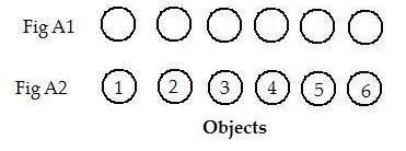
It is necessary to distinguish objects, one from another. To do this assign numbers to objects as names. In Fig A2 the six objects have been assigned natural numbers (positive integers) 1,2,3,4,5,6 and are called integer-names. It is important that zero and negative integers never be chosen as integer-names of objects, because those numbers will have special meanings for the computer in later constructions. If there are exactly n objects involved then the consecutive numbers 1,2,...,n are usually chosen in one-to-one fashion as names to the objects. It will be convenient later if all isolated objects that have no connections have been assigned the largest integers. Other than these two suggestions there is ususlly no significance to the asignment of integer-numbers to objects: any object can be assigned 1, any other assigned 2,... etc. and n is assigned as the last object, if there are exactly n objects.
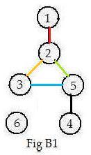
Usually some, perhaps all, of pairs of objects are linked together. In drawings the links are represented by simple line segments or curves joining the objects as end-points. (See Fig B1 below.) The lengths of the line segments or curves between objects are not important, only their existence. In these discussions such connections will be called links. (In some textbooks they are called edges.) In Fig B1 the two objects 5 and 3 are linked together. A total of five pairs of objects are linked together with five links. Some objects are involved with more than one link. For example, object 5 is linked to objects 2,3 and 4. In an undirected graph the the connections are bi-directional. This means that object 5 is linked to object 3, and also object 3 is linked to object 5. In discussions the objects with numbers and connections between them are written as 5-3 without the circles around the numbers as in drawings. Using this notation the two linked pairs (the second pair is the reverse of the first pair)
The computer, however, will consider the link in 5-3 as directed (5→3). In programs that require bidirectional links, it will produce from it the reverse 3-5 (3→5) if it does not already exist. The two symbols 5-3 and 3-5 together will represent a bi-directional link in the computer.
The idea of a link between two objects plays a fundamental role in graphs. As a result of its importance various definitions about a linked pair of objects have been made. Looking at Fig B1, it seems that object 2 is closer to object 5 than object 1 is to object 5.
[1.1] (Adjacent objects) Two objects are linked together or adjacent if
(a) the connection is bi-directional: each object is connected to the other, and
(b) no other object is involved in the connection between them.
Adjacent objects are called neighbors of each other. It is a mutual (symmetric) relationship. In Fig B1, object 2 is a neighbor of object 5 and 5 is a neighbor of 2.. But object 1 is not a neighbor of object 5. There is no single link between objects 1 and 5.
It is quite possible that an object not be linked to any other object. Then it is called isolated. Isolated objects have no neighbors. For example, object 6 has no neighbors. The concept of neighbors needed a picture of a graph to motivate it.
However useful for human understanding, it is not practical that the drawing of a graph serve as a direct source of data for a computer. Then what data can be collected from the drawing and given to the computer? Obviously the data will be integers. Since every object has an integer-name, the computer accepts objects from the graph by accepting their integer-names. It is easy to write a program that accepts the linked objects 2-5 where the computer recognizes 2 as the first and 5 is the second integer.
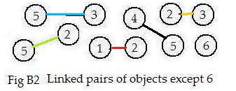 This discussion suggests that a list of all the linked pairs in a graph may be used as input to a computer. Therefore, tear apart the graph in Fig B1 into a collection of linked pairs
Since links here are bidirectional there is no loss of data if the end points of some linked pairs are interchanged. The computer does this and sorts the results to change (*) to get
Click here for details how to prepare lists of links for input to a computer.
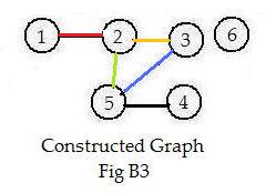
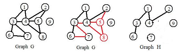
An interesting but instructive curiosity is the fact that in a drawing the linked pairs in B2 can be assembled in different directions to produce the graph in Fig B3. Conversely, the graph B3 can be disassembled to produce the links in B2. The two graphs B1 and B3 are said to be "(topologically) equivalent." The links in Figures B1, B2, B3 are color-coded to show the same links in all three figures.
To preserve the simplicity of all links between objects, discussed and shown in this volume, restrictions are imposed on them:
 [1.2] (Restrictions) In any complete collection of links and objects:
(a) only a finite number of objects are involved; (Usually the number is small.)
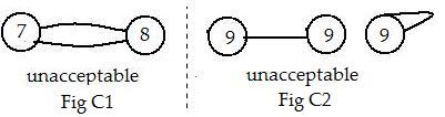
(b) never more than one (bi-directional) link connects two objects: 7=8 is not allowed. (Fig C1)
(c) never is there a link between an object and itself: 9-9 is not allowed. (Fig C2)
Logically, isolated objects satisfy both conditions (b) and (c). Therefore, isolated objects are allowed.
Everything in the collection of links and objects in Fig B1 are allowed.
The two links in C1 are bidirectional, and not allowed.
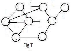 Discussions above present graphs with objects already having integer-names. But a graph can exist without these numbers. Fig T is such a unlabeled graph. People without communication between them might give different integer- names to the objects (from N8) to copies of the graph. But on all copies, the number of objects is 8. The number of links is 13. There are 4 neighbors of the object on the extreme left. These properties of the graph would be the same for the graphs before the two people, because the properties exist independently of any integer-names given to the objects.
 [1.3] (Not dependent upon labels) Any property of a graph that does not change if the objects receive any different integer-names is said to be independent of labels.
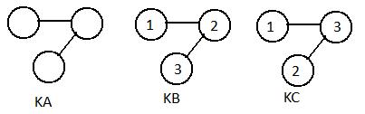 In the adjacent figures the objects in the unlabelled graph KA have been given the same triple of natural numbers in KB and KC. The statement "object 1 and object 2 are linked" is true in KB but not in KC. Therefore, that statement is dependent upon what labels are used on objects. Any numbering placed on all objects is a convenience, and replaces awkward phrases like "the object on the extreme right." But the numbering is not a part of the intrinsic structure of the graph.
Each object in a graph has neighbors. Neighbors are part of the structure of a graph and hence are independent of labels. The number of neighbors an object has, is called the degree of the object. In figure KC above object 3 has degree 2. But object 2 in KC has degree 1. An object is isolated if and only if it has degree 0.
If the graph is disassembled into a collection of linked pairs of objects (and isolated objects) any numerical labels that were given to all objects tell what end objects of linked pairs are to be joined together and the graph can be reconstructed. However, the reconstructed graph may or may not look like the original graph. But the two graphs are related.
[1.4] (Equivalent graphs) One graph is equivalent (or isomorphic) to another graph with the same objects if the first graph can be disassembled into a collection of linked pairs of those objects, and from all of these same linked pairs the other graph can be constructed.
Of course, the links in the collection may be expanded or shortened.
The graphs B1 and B3 show that equivalent graphs when drawn need not be congruent figures.
This definition is incomplete. If the integer-names have been assigned already to all of the objects in the second graph, those names may be different from the ones obtained from the assembling process. Also the disassembling one graph and assembling and construction of the other graph is usually difficult if there are many objects and links involved. A better definition will be discussed in a later chapter of this volume. But let [1.4] stand for now.
If some graph represents a grid of telephone poles with wires connecting them, then any equivalent graph represents the same grid.
It is quite possible that the collection of linked pairs from the decomposition of one graph cannot in any way be used to construct a second graph. For example, the collection may have too many pieces or not enough pieces in it. The following give some of the obvious reasons:
[1.5] (Non-equivalent graphs) Two graphs cannot be equivalent if
(a) one graph has more objects than the other.
(b) one graph has more links than the other.
(c) one graph has more isolated objects than the other.
<
[1.6] The following are the general instructions for deriving the short adjacency array from a drawing:
(a) For each object locate all of its neighbors.
(b) Delete all neighbors whose integer names are less than the integer-name of the object.
(c) Write the negative of the integer-name of the object and after it write all the undeleted integer-names (natural numbers) of the neighbors.
Note1: if all the integer-names (natural numbers) of the neighbors have been deleted, do not write the (negative of the) integer-name of the object in the array.
Note2: if the object is isolated, then write only the negative of its integer-name, with no natural numbers immediately after it.
(d) Enclose the entire graph array in brackets.
Click here for practice deriving the short adjacency array directly from a drawing of a graph. Because of its convenience the simple adjacency array will be the most used form for input of data from a drawing of a graph into the computer.
A graph is completely determined by what objects are neighbors of each object. But because of rule [1.6b] the short adjacency array usually does not give all of the neighbors. Using only rules (a) and (c) the long adjacency array for B1 is
     1   2   3   4   5   6
 1   0   1   0   0   0   0
 2   1   0   1   0   1   0
 3   0   1   0   0   1   0
 4   0   0   0   0   1   0
 5   0   1   1   1   0   0
 6   0   0   0   0   0   0
The rows reveal all the neighbors of an object. In row 2 there is a 1 under 1,3,5. This is equivalent to the cluster -2,1,3,5 in the long adjacency array (****). The adjacency matrix is equivalent to the long adjacency array of a graph.
The red matrix is symmetric about the diagonal of all zeros because links are bi-directional: if x is linked to y then y is linked to x. The red table is called the adjacency matrix for graph in Fig B1. And the same matrix is the adjacency matrix for graph in Fig B3.
In general, if a graph has n objects then its adjacency matrix will be a square symmetric matrix of size nxn. But as data for inputting a graph into a computer it is large, tedious and prone to errors to prepare before input, e.g. a misplaced 1 or 0 may happen.
Being equivalent is truly an equivalence relation between graphs.
(reflexive) It is possible to disassemble a graph into a collection of linked objects and reassemble them to get the same graph back
(symmetric) If one graph is disassembled into a collection of linked objects and the collection assembled to produce the second graph, then reversing the steps disassembles the second graph and assembling produces the first graph.
(transitive) If one graph is disambled into link objects and assembling them to produce a second graph, then disassembly of the second graph produces the same linked objects and assembly of them produces the third graph, then the same collection of linked objects can be used from disassembly of the first graph to produce the third graph.
[1.7] Two graphs constructed from the same collection of objects and links are equivalent. It is possible for two graphs to be equivalent even if they are constructed from different collections of objects and links. One collection is obtained from the other by using different assignments of distinct integer-names (a permutation of natural numbers). A discussion of equivalent graphs is given in a later section of this volume F.
There are two extremes of linkage in graphs:
(no links) Every object is isolated; no links appear anywhere. Such a graph may be called discrete. Graphs remaining discrete have almost no interest.
(all objects linked together) Every pair of objects are linked. A graph satisfying this condition is called complete.
It is trivial but true that every pair of discrete graphs with the same number of objects are equivalent.
Two complete graphs with the same number of objects are equivalent, because they produce the same table of neighbors. In the adjacent figures are two complete graphs of four objects.
Notice that the number of neighbors of any object equals the number of links drawn to that object. Since each object has 3 neighbors and there are 4 objects, it may seem that there should be 4x3=12 links. But each link is counted twice in that product, because being neighbors is a mutual relationship. Therefore, there are 12/2 = 6 links. Notice that links can cross and their intersections are not where objects are.
In a complete graph of n objects each object has n-1 neighbors. Therefore, (since each neighbor has been counted twice)
[1.8] (Links in a complete graph) In a complete graph of n objects there are n(n-1)/2 links.
Statement [1.8] provides an upper limit on the number of links in a connected graph.
The argument supporting statement [1.8] shows the nature of some arguments in graph theory, indeed, in finite mathematics. They are informal and therefore differ in style from formal proofs in traditional plane geometry.
It is possible that a set exists within a set. Then the first set is called a subset of the second set. Similarly, a group may exist within a group. So the first group is a subgroup of the second. A graph may exist within a graph. The only objects in the first graph are objects in the second. Similarly, all of the links in the first graph are also links in the second graph. Intuitively speaking, the subgraph "inherits" objects and links from the main graph.
[1.8] (Subgraph) A graph H is a subgraph of a graph G if and only if H satisfies the following conditions:
(a) all the objects in H belong also to G;
(b) If a link is in H then it must exist in G and both objects connected by that link are in H.
Condition (b) prevents cutting a link. Not allowed is an object and part of its attached link be in a subgraph and the remaining part and object be outside the subgraph. However, the link can be excluded from the subgroup, while an end object or both may be in the subgraph.
In the adjacent Fig E is a graph G, another graph G and a graph H. Some of the links and objects in the second graph became red. They are to be removed to produce graph H. Then H is a subgraph of G. The construction of H (by partial distruction of G?) introduced no other object or link outside G into H.
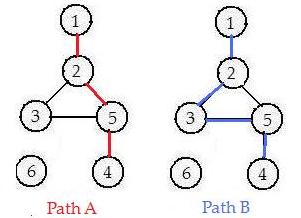 In the adjacent figures, objects 1 and 4 are not linked. No single link connects them, yet a bug following some consecutive links could go from object 1 to object 4 (or from object 4 to object 1). He could do it by passing through objects 2 and 5 (Path A). He could also do it by passing through objects 2, 3 and 5 (Path B). More exactly, the two forms
[2.1] (Graphical sequences) A graphical sequence of objects and links is a subgraph satisfying the following conditions:
(a) The number of objects and links are finite.
(b) Between every pair of adjacent objects in the sequence is a link.
(c) No object has more than two links attached to it.
(d) No object appears more than once in the sequence. (The sequence is said to be simple.)
It will be convenient to allow any isolated object by itself to be a path. It satisfies conditions (a), (c), (d). Logically, it does not violate condition (b) because there are no existing adjacent objects without a link.
There are two important graphical sequences in graph theory. They are defined in [2.2] and [2.4] below.
[2.2] (Paths) A (simple) path connecting two distinct objects is a graphical sequence with those two objects as ends. (Ends have only one link attached to them; all other objects have two attached links.)
Paths have the following properties:
(a) Every path is a subgraph of a graph.
(b) No object in a path has more than two links attached to it.
(c) A link is a path between the two objects that it joins.
(d) In every path joining two distinct objects, the number of objects is one more than the number of links.
(e) Paths have no breaks or interruptions along their entire lengths.
Statement (e) makes a path an important tool in graph theory. It motivates the following trivial definition:
[2.3] (Connected objects) Two objects in a graph are connected if there is a path with them as ends.
Intuitively speaking, suppose that the two given objects in [2.2] become a single object, i.e they coincide. Then the graphical sequence connects the object with itself. It is possible to go from the given object through the other objects and come back to the given object. In the adjacent figure the object 2 is connected with itself. In order to do this, each object there is directly connected with two other objects (neighbors).
[2.4] (Loops) A loop is a graphical sequence in which every object in it is linked with exactly two other objects in it.
 A loop is also called a cycle in some text books.
It is not possible to represent a loop with graphical sequence on a single horizontal line without repeats of objects. Therefore, it will be represented as a sequence with equal ends:
Equally valid for the same loop is the notation 5-8-3-9-2-5.
In every loop there is the same number of links as objects. The only possible difference is that motion might seem to go clockwise for one notation and counter-clockwise for the other notation. But in this volume directed motion will not be significant because links everywhere are bi-directional.
In any physical loop the minimum number of objects is three, and therefore the minimum number of links is also three.
In the loop under discussion objects 8 and 9 are not neighbors. A bug can go from object 8 to object 9 along either of two paths:
[2.5] A loop exists if and only if two different paths connect the same pair of objects.
Two paths connecting the same two objects might be considered equivalent (but not equal). Either path proves that the two objects are connected.

In the adjacent figure the same bug can choose among four paths to take him from object 8 to object 9. There are more than three loops. May the reader find them all.
Notice the hazzard that loops present to the travelling bug and the computer program simulating the bug. Both may traverse any loop infinitely many times, never leaving it, unless precautions are taken. This is a problem that loops may present.
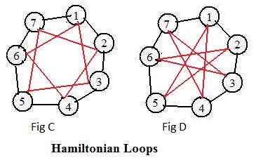
In some graphs, but not all, special paths and loops exist. A loop in a graph is Hamiltonian if it contains all objects in the graph once and only once. In the adjacent figure are two graphs. Each has 7 objects. Also, each has two Hamiltonian loops, one black the other red.
In Fig C, 1-3-5-7-2-4-6-1 is one Hamiltonian loop. Let the reader write down two more Hamiltonian loops.