Additional Material for this Chapter
Exercises for this Chapter
Answers to Exercises
Computer Programs
Return to index of all chapters in this volume
Volume F Chapter 2
Ugraphs and Weights
Section 1: Connected Ugraphs and Components
With ocean between them the roads of the United States, the roads of England and the roads of Australia are separated, because there are no roads that connect them together. In Fig A2 below there exists a similar situation in that graph, namely three separated "pieces." But the roads of southern Alaska and the roads of the continental US are not separated. There is a road connecting them (through Canada). Using this road there can be found a road between any city in the continental US and any city in southern Alaska. The following definition is motivated by this remark and Fig A1, where the graph is in one piece:
[1.1] (Connected Graphs) A Ugraph is connected if and only if for any pair of nodes in it there is a path connecting them.
A path may be a single link, but more often it is composed of a chain of links joined together at nodes. In Fig A1 there is a path between node x and node y, and a path between node y and node z. Therefore, there is a path between node x and node z. These three paths make the graph connected.
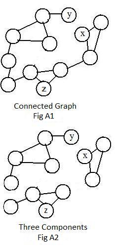
There may be more than one path connecting a pair of nodes. There must be at least one path connecting any pair of nodes in a connected graph.
If a graph is connected then in a drawing it appears to be in one piece.
Certain links in the graph in Fig A1 were deleted to produce the graph in Fig A2. Those deletions separated the graph into three connected pieces, called components. They contain nodes x,y and z. The component containing node x has 3 nodes in it. The component containing nodes y and z have 5 and 4 nodes respectively. The three components together contain all the 12 nodes in the original graph.Although there are three pieces (subgraphs), the entire drawing of Fig A2 is a single graph.
Notice that the largest connected subgraph containing the node y in Fig A2 is the component containing 5 nodes. This observation suggests another way of defining a conponent, as the connected subgraph containing the most nodes.
The adjacent drawing Fig W2 shows graph in Fig A2 with labels (where x=6, y=2, z=5). The input-data (containing the short adjacency array) for W2 is:
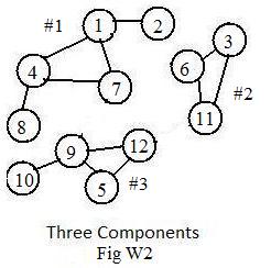 [U"Fig W2" (1),2,4,7, (3),6,11, (4),7,8, (5),9,12,
(6),11, (9),10,12]
[U"Fig W2" (1),2,4,7, (3),6,11, (4),7,8, (5),9,12,
(6),11, (9),10,12]
The separation of components has no effect on the array.
Adding links 8-10 and 11-12 to the graph in Fig W2 produces Fig W1 (not drawn here) whch is Fig A1 with labels. The graph data for Fig W1 is obtained by including clusters (8),10 and (11),12 in the graph data for Fig W2.
After accepting the graph data for Fig W2, the computer names the components #1, #2, #3 and prints out all the nodes in each component:
***
Ufile Fig W2 12 Nodes 12 Links
Component #1: 1 2 4 7 8
Component #2: 3 6 11
Component #3: 5 9 10 12
Location of (nodes) in components
(1)1 (2)1 (3)2 (4)1 (5)3 (6)2 (7)1 (8)1 (9)3 (10)3 (11)2 (12)3
The last line shows that node (5) is in component #3.
If the computer accepts the graph data for Fig W1 then it prints out component #1: then all 12 nodes in the graph. If there is only one component then the graph is connected.
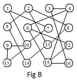
In some graphs like in Fig B the components are so intertwined (yet disjoint) that it is diffiicult to identify immediately the components visually from the drawing. The computer may come to the rescue after labels have been assigned to all the nodes.
[1.2] (Characteristization of components) All the components of a Ugraph form a partition of the graph into separated connected subgraphs.
A very simple proof of [1.2] exists if every node is allowed to be connected to itself, even if there is no visible loop containing that node. Then the relation
node x is connected to node y
on a graph is an equivalence relation:
(reflexive) every node is connected to itself;
(symmetric) if a first node is connected to a second node, then the second node is connected to the first node (paths are bidirectional);
(transitive) if a first node is connected to a second node, and the second node is connected to a third node, then the first node is connected to the third node (join paths at the second node).
The equivalence classes formed from this relation are the connected subgraphs. Two nodes are in the same component if and only if some path in the component connects them.
Intuitively speaking, components are disjoint and can be considered as isolated pieces of the graph. No links or paths join them (recall isolated nodes).
Also, the component containing a given node is the largest connected subgraph containing that node.
It goes without saying that a graph is connected if and only if there is exactly one component containing the whole graph.
There are various ways of identifying any component of a graph. In increasing information about the component:
(a) Pick a labeled node in the component, and identify the component as the component containing that node.
(b) In a labeled graph, use the (#) number that the computer assigns to that component.
(c) In a labeled graph, list the labels of every node in that component.
(d) In a labeled graph, give the adjacency array for that component.
Most graphs under discussion in the rest of this volume will be connected.
***
Starting with a collection of N isolated nodes, attach links one at a time to pairs of nodes. When does the resulting graph become connected? Is there a minimum number of links needed?
Label the nodes with natural numbers 1,2,...,N. Then form the path
1 - 2 -3 - ... - N
There are N-1 links in this path. The path connects all nodes in the collection. Any fewer links will not connect all the nodes. Actually, a proof, not given here, can be made using mathematical induction. That proof supports the following:
[1.3a] (Minimum number of links in a connected graph) A connected graph with N nodes cannot have less than N-1 links.
For example, if a graph has N =5621 nodes and only 4003 links then that graph cannot be connected, because 4003 is less than the minimum number N-1 = 5620.
The following statement is equivalent to [1.3a]:
{1.3b] (Too few links in a graph) If a graph has N nodes and less than N-1 links, then the graph cannot be connected.
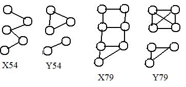 Notice that statement [1.3b] says nothing about a graph with N nodes having exactly N-1 or more links. The adjacent four graphs show that [1.3b] gives no definite answer for such graphs.
In Fig X54 the graph has 5 nodes and 4 links (exactly the minimum 4), and the graph is connected. But in Fig Y54 there are 5 nodes and 4 links and the graph is not connected.
In Fig X79 the graph has 7 nodes and 9 links (more than the minimum 6), and the graph is connected. But in Fig Y79 there are 7 nodes and 9 links and the graph is not connected. It is an interesting fact that loops must be involved to produce some of these counter-examples.
Because the numbers of nodes and links in the following two statements do not satisfy the conditions of [1.3b] that statement [1.3b] cannot be used to give more definite answers to them:
If a graph has 5621 nodes and exactly 5620 links the graph may or may not be connected.
If a graph has 5621 nodes and exactly 6054 links the graph may or may not be connected.
Section 2: Trees
In this section a very special and important kind of graph is discussed. Previous discussions commented negatively about loops in graphs. In this section no graphs have loops. Furthermore, the graphs are connected. These two conditions lead to the following definition:
[2.1] (Trees) A tree is a connected Ugraph without any loops.
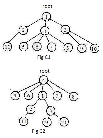
The graphs in Fig C1 and Fig C2 are trees. Because of the name the graphs are presented as upside down trees with specific nodes called roots on top.
The graph in Fig C1 has the following short adjacency array:
(1),2,3,4, (2),11, (3),9,10, (4),5,6,7,8
In Fig C2 the root is node 4. The short adjacency array for it is
(1),2,3,4, (2),11, (3),9,10, (4),5,6,7,8
Therefore the two graphs are (label) equivalent. This indicates that any node in a tree may serve as a root. However, if a tree is unlabeled then it may seem natural, but not necessary, to label the root node 1.
A graph is a tree if and only if every pair of nodes is connected by a single path. Going down a tree a final node (dead end) must be reached. As a result there must be some nodes with degree 1. In a drawing such nodes are part of the tree with a single link. They are often called leaves. In Fig C1 all seven leaves have labels larger than 4.
Notice that the integer-names of leaves need not appear in parentheses in the small adjacency array.
Sometimes it is necessary to consider graphs that are not connected. Those graphs cannot be trees, but their components may be trees. A graph is called a forest if and only if all of its components are trees. Usually more than one component exists for the word "forest" to be used.
By going down a path from the root of a tree, various links are traversed. Sometimes it is useful to count the number of links in that path. In this volume the number of links in a path is called the graphical length of the path. It does not truly measure the physical length of the path because the graphical length does not involve the physical lengths of the contained links, only the number of links.
For any node in a tree there is a single path between it and the root. The graphical length of that path is called the level of the node. Of course, the level of any node depends upon which node is chosen as root. But the root is always at level 0.
In both Fig C1 and Fig C2 the graphs show nodes at the same levels. But in Fig C2
Level 0: node 4
Level 1: nodes 5,6,1,7,8
Level 2: nodes 2,3
Level 3: nodes 11,9,10
Levels form a partition of the tree with an assigned root. In fact they are equivalence classes produced by the relation "node x is at the same level as node y".
For any given node in an upside down tree, the neighbors of that node are either above it or below it. If the given node is linked to another node above it. then that second node is called the parent of the given node. The given node may be linked to nodes below it. Each of those nodes is called a child of the given node. In Fig C1, node 1 is the parent of node 4, and nodes 5,6,7,8 are children of node 4.
In every upside down tree there are nodes (leaves) without children. In both figures C1 and C2 nodes 5,6,7,8,9,10,11 have no children. Such nodes are considered parents without children. Also, every node has exactly one parent, except the root. Node 1 in Fig C1 and node 4 in Fig C2 have no parents. It will be convenient to "invent" an artificial parent for any root node. It will have the integer-label 0 (zero). An artificial link connects node 0 to the root node. The artificial node and link are called pseudo-node and pseudo-link respectively. They are not really parts of the tree, but they do allow the following statement to be made:
[2.2] (Single parent) In every tree with one node selected as a root node, every node in it has exactly one parent.
For these two graphs the computer may print out the following long adjacency array (LAA) and tree adjacency arrays (TC1, TC2) which display different roots:
	      LAA		     TC1		    TC2
	(1),2,3,4		0,(1),2,3,4		4,(1),2,3
	(2),1,11		1,(2),11		1,(2),11
	(3),3,9,10		1,(3),9,10		1,(3),9,10
	(4),1,5,6,7,8           1,(4),5,6,7,8           0,(4),1,5,6,7,8
	(5),4  	     		4,(5)  			4,(5)
	(6),4  			4,(6)  			4,(6)
	(7),4  			4,(7)  			4,(7)
	(8),4  			4,(8)  			4,(8)
	(9),3  			3,(9)  			3,(9)
	(10),3			3,(10)			3,(10)
	(11),2			2,(11)			2,(11)
(The computer may print out arrays horizontally.) Looking at columns TC1 and TC2, the parent of each (node) appears before the (node). Zero appears before the root node. The children, if any, appear after the (node). In this way, TC1 and TC2 reflect the root and the structure of an upside down tree, while the long adjacency array LAA does not.
It turns out that the sequence of all parents determine completely the structure of a tree with a root. From the sequences of parents in TC1 and TC2, namely,
0,1,1,1,4,4,4,4,3,3,2
4,1,1,0,4,4,4,4,3,3,2
The computer can construct the entire arrays TC1 and TC2, respectively. (To input these sequences, the computer will ask for the parent of each node 1,2,...,11, but not ask for any children.) The following summarizes this discussion:
[2.3] (Parents determine a tree) For a graph if a node can be chosen as a root and every node (except the root) has a single parent, then the graph must be a tree.
By going up the links to parents, a path is formed connecting any node to the root node. Since the parents are unique, no two paths connect the node to the root, so no loops exist in the graph.
***
 In some trees not many links contact the nodes.
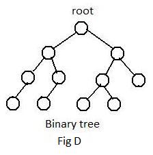
[2.4a] (Binary trees) A tree with a root is binary if every node is a parent of 0, 1 or 2 children.
Fig D shows an unlabeled binary tree with a root. A more general definition with no mention of roots [5.4a], but less intuitive, is
[2.4b] (Binary trees) A tree is binary if every node has a degree less than 4.
All of the nodes in Fig D have degree less than 4. No degree can be zero because by definition a tree is always connected.
The tree in Fig C1 is not binary. Node 4 in that graph has degree five, violating the conditions given in [2.4b].
Binary trees are used in a number of places in mathematics. They may be used to sort a sequence of numbers into increasing order. Click here to see the discussion. Another use for trees is in game theory. Click here to see how a tree gives support to a strategy of always winning in a simple game called "Game of Eight."
***
Section 3: Weights, their Interpretations and Input-data
In the previous chapter natural numbers have been used as names of nodes, and placed inside the circles representing nodes. In this chapter numbers in the drawings will be placed along side of links and nodes for different purposes. Collectively they are called weights, but they will receive more specific names when their graphs reflect real situations. Unlike the natural numbers used as names to identify nodes, weights come as fixed data that are considered parts of the graph. In these discussions a graph with weights is different from the same graphical structure without weights.
In discussions in this section the graphs are deliberately small for the purpose of immediate understanding. However, in later sections it will be much more convenient to use the computer with the larger weighted graphs (limited to 50 nodes or less). Therefore, nodes in unlabeled weighted graphs eventually will receive integer-names.
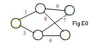 A most easily understood idea is distance between objects, such as cities and towns. It is a positive real number, but here it will be rounded off to the nearest natural number. In Fig E0 the unlabeled nodes represent five towns and the links represent simple roads joining adjacent pairs of towns. The physical lengths of these roads assign natural numbers to all links. (In drawings the links are not drawn with lengths equal or even proportional to these natural numbers given to them.) In these discussions numbers given to links will be in red, to distinguish them from black integer-names given to nodes (and written inside them).. The numbers may have a different interpretation, say, cost in dollars, or time to travel the link, for transportation service between adjacent towns. But distances are the most natural interpretation of values given to links. A graph with such numbers associated with its links is called in these discussions a graph with weights on its links, or simply a weighted graph if there will be no confusion.
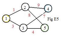 Asssign integer-names to the nodes in graph E0 to produce graph E5. Ignoring for the moment the weights given to the links, the short adjacency array for graph E5 is
(1),2,3, (2),4,5, (3),4,5
The short adjacency array with weights as input-data is
(*) [UL"E5"
(1),2,3,#1,3, (2),4,5,#9,8, (3),4,5,#7,5]
The letter L just after the U tells the computer that later numbers after # will be associated with Links to neighboring nodes written just before #. Therefore, there must always be the same number of weight numbers after the # as neighboring node numbers before the # in each cluster.
Notice: The short adjacency array, and not the long adjacency array, should always be used in the input-data to the computer when weights are involved.
Although the imput data (*) above can be typed onto the data file directly, it is better to use an input program. There is much less chance of making a mistake with all the required punctuation and spaces. It is much easier to use the input program. As usual the program will first ask for the name of the data-input. (For this graph the name is 'Fig E5'.) Then it will ask for the number of nodes. (The number is 5.)
The input section of the program is in two parts, (Part A) input-data for the short adjacency array and (Part B) input-data for the weights on links. (No color other than black is used in anything that the computer reads or writes.)
Part A: The neighbors with higher labels than given (nodes) are typed in answer to the computer's statements:
the neighbors with higher numbers than (1) are: 2,3
theneighbors with higher numbers than (2) are: 4,5
the neighbors with higher numbers than (3) are: 4,5
the neighbors with higher numbers than (4) are:
the neighbors with higher numbers than (5) are:
Part B: The needed weights on links are typed in answer to the computer's statements:
the weight on link 1-2 is: 1
the weight on link 1-3 is: 3
the weight on link 2-4 is: 9
the weight on link 2-5 is: 8
the weight on link 3-4 is: 7
the weight on link 3-5 is: 4
Combining the node (integer-names), node neighbors and weights produces the colorful short adjacency array:
(1),2,3, #1,3, (2),4,5, #9,8, (3),4,5, #7,4
The input-data has the form
[UL"E5" (1),2,3, #1,3, (2),4,5, #9,8, (3),4,5, #7,4]
The # separates the numbers on the links from the neighbors of the (node). The L just after the U tells the computer that the links have weights. Without the L the computer would ignore the # and the numbers after it. Therefore, the computer would thinik that the graph had no weights.
After the computer receives and processes the data for the weighted graph it will print for verification without colors:
Input-data containing a short adjacency array with weights on links =
[UL"E5" (1),2,3, #1,3, (2),4,5, #9,8, (3),4,5,#7,4, (4), (5)]
***
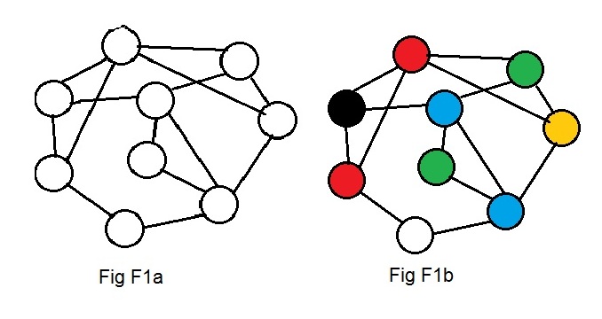
Weights may be assigned to nodes. They are non-negative integers in discussions here. Weights on nodes have interpretations that are very different from those for weights on links. The most intuitive interpretation involves colors. Fig F1a shows an unlabeled graph. Fig F1b shows some of the nodes having colors, but the graph remains unlabeled. The computer cannot accept colors as input data. Away is needed to represent colors that is acceptable to the computer.
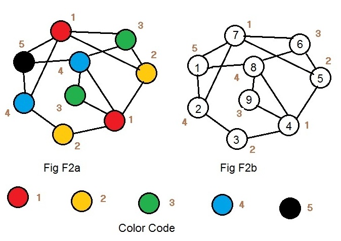 In Fig F2a the same colors are used but fill some different nodes. Along side each colored node is a natural number. Along side every red node is the number 1. Along side every yellow node is the number 2. Every node with the same color has the same natural number beside it. Below the graph in Fig F2a is the array revealing the color codes. In Fig F2b the colors have been removed and natural numbers 1,2,3,4,5 have been assigned to the nodes. This this is a labeled graph with weights on its nodes, or simply a weighted graph if there will be no confusion.
Only from the graph in Fig F2b can input-data for the computer be formed.
The input section of the program is in two parts, (Part A) input-data for the short adjacency array and (Part B) input-data for the weights on nodes. (No color other than black is used in anything that the computer reads or writes.)
Part A: The neighbors with higher labels than given (nodes) are typed in answer to the computer's statements:
the neighbors with higher numbers than (1) are: 2,7,8
theneighbors with higher numbers than (2) are: 3,7
the neighbors with higher numbers than (3) are: 4
the neighbors with higher numbers than (4) are: 5,8,9
the neighbors with higher numbers than (5) are: 6,7
the neighbors with higher numbers than (6) are: 7,8
the neighbors with higher numbers than (7) are:
the neighbors with higher numbers than (8) are: 9
the neighbors with higher numbers than (9) are:
Part B: The needed weights on nodes are typed in answer to the computer's statements:
the weight on node 1 is: 5
the weight on node 2 is: 4
the weight on node 3 is: 2
the weight on node 4 is: 1
the weight on node 5 is: 2
the weight on node 6 is: 3
the weight on node 7 is: 1
the weight on node 8 is: 4
the weight on node 9 is: 3
Combining the node (integer-name), node neighbors and weight produces the input-data:
[UN (1),2,7,8,#5, (2),3,7,#4, (3),4,#2, (4),5,8,9,#1, (5),6,7,#2, (6),7,8,#3, (7), #1 (8),9,#4, (9),#3]
For each (node) there is only one weight because each (node) has only one color. Should some node not be colored then the computer gives it a color code of 0 (zero). This is equivalent to saying that the code color for white is zero. See Fig F1a and Fig F1b.
Section 4: Spanning Trees of Shortest Distances
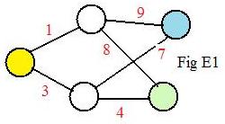 In the previous section Fig E0 showed an unlabeled graph with weights on the links. In the adjacent drawing E1 is that same graph except three of the nodes are colored.
Paths from the yellow node to the other colored nodes are of interest. Since it is natural to define the length of a path as the sum of the lengths (weights) of all the links in it, the lengths of two paths connecting the yellow and green nodes are
3 + 4 = 7 and 1 + 8 = 9.
The shorter path is shown in the lower part of Fig E2 with think black links. There are no shorter paths in the graph between those two nodes.
In the previous section Fig E0 showed an unlabeled graph with weights on the links. In the adjacent drawing E1 is that same graph except three of the nodes are colored.
Paths from the yellow node to the other colored nodes are of interest. Since it is natural to define the length of a path as the sum of the lengths (weights) of all the links in it, the lengths of two paths connecting the yellow and green nodes are
3 + 4 = 7 and 1 + 8 = 9.
The shorter path is shown in the lower part of Fig E2 with think black links. There are no shorter paths in the graph between those two nodes.
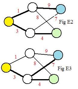 There are a pair of paths connecting the yellow and blue nodes. Their lengths are
1 + 9 = 10 and 3 + 7 = 10
Both of them are the shortest paths.
Fig E2 shows the first path connecting the yellow and blue nodes along the upper part of the graph, while Fig E3 shows the second path with thick black links.
A path of minimal length between two nodes is a path that has the shortest length. It may also be called a minimal path.
It is called a minimal path and not "the minimum path" because there may be other paths with the same shortest length, as between the yellow and blue nodes.
Expand the search for minimal paths from the yellow node to all the other nodes in graph E1. In Fig E2 is one solution.
The minimal paths to the white nodes are parts of the minimal paths to the green and blue nodes.
Another solution is shown in Fig E4.
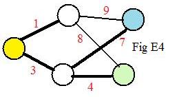 Notice that the blackened links and nodes in Fig E2 and Fig E4 fit the definition of spanning trees on the same graph in Fig E0. If there are two minimal paths between the same two nodes then only one minimal path is selected (by the computer) to be in the spanning tree.
[4.1] (Spanning trees of minimal paths) The collection of all minimal paths from a single node to all other nodes in a connected Ugraph form a spanning tree on the graph. That single node becomes a root of the tree.
Section 5: Coloring of Nodes
----------------------------------
Situation A:
Five containers hold chemicals. Two containers are incompatible if a mixture of their contents is dangerous, an explosion or poisonous gas occurs. It is desirous to store all containers in cabinets, but no dangerous chemicals are in the same cabinet.
A trivial solution: store each container in a different cabinet. Then five cabinets will be needed.
But suppose not all pairs of containers contain chemicals that are dangerous when mixed. Then there is a more economical solution that requires fewer cabinets.
----------------------------------
Situation B:
Five persons from different countries will be seated at dinner tables. But some countries are at war with other countries. Two people are incompatible if their countries are at war with each other. Incompatible people will not sit at the same table.
A trivial solution: seat each person at different tables. Then five tables will be needed.
But suppose not all the countries are at war. There are some pairs of countries that are friendly. The people from those coutries are willing to sit at the same table. There is a solution that requires fewer tables.
----------------------------------
Situation C:
Five TV stations are ready to broadcast signals to a city. They must be assigned channels. Stations are incompatible if given the same channel, their signals interfere with each other (their transmitters are too close or too powerful).
A trivial solution: assign a different channel to each station.
But suppose not all stations produce signals that interfere with each other. Some transmitters are far enough apart. Fewer channels are needed.
----------------------------------
In this section the method for finding compatible objects (or people) is to exclude all the pairs of incompatible objects. A list of pairs of incompatible objects is given, those objects and their incompatibilities are represented by linked nodes in a Ugraph. Nodes that are not directly linked (but are connected) are compatible. More details are needed. The method will be carried out by drawings of graphs, and later by computer.
Give the objects ( containers, people, stations) in the above situations integer-labels 1,2,3,4,5. Make list of all incompatible objects usiing these labels:
1,2 1,4 1,5
2,1 2,3 2,5
3,2 3,4
4,1 4,3
5,1 5,2
Represent the objects by labeled nodes (Fig Gx). Then linked every pair of nodes that represent incompatible objects (Fig G0). Those nodes are also called incompatible.
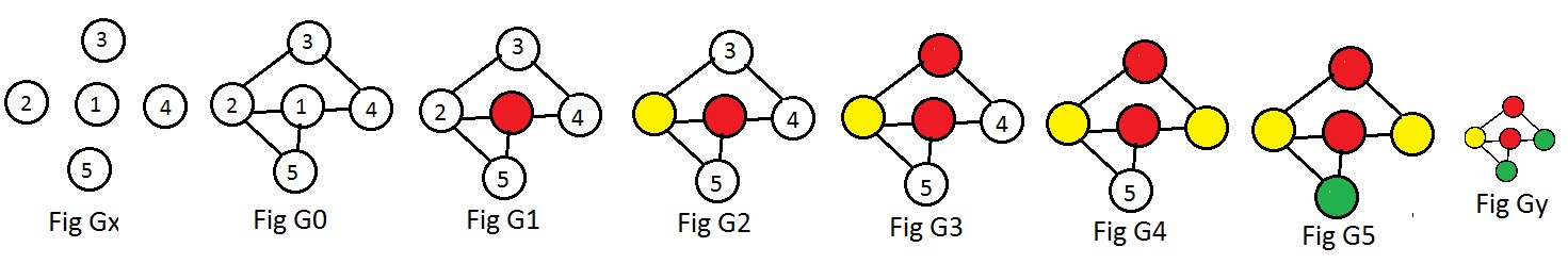 The nodes will receive colors in the order of their integer-labels. However the following rule will be observed:
[5.1] (Coloring Rule A) For any coloring ofl nodes in a Ugraph, every pair of nodes that are linked together must have different colors.
In other words, incompatible nodes must have different colors. A trivial solution that always satisfies Coloring Rule A give each node a different color. Then five colors will be needed. If the graph is not complete, then there exist pairs of nodes without links joining them. There is a waste of colors, because these nodes may receive the same color and not violate Coloring Rule A. The following additional rule will be observed to reduce trivial colorings and economize on the number of colors needed:
[5.2] (Coloring Rule B) Use as few colors as possible.
The smallest number possible is called the chromatic number of the graph. (Its existence is guranteed by the well ordering principle for the set of natural numbers.) For large graphs with many nodes and links this number is usually difficult, if not impossible, to find even with the help of a high-speed computer.
In graphs G1, G2, G3, G4, G5 nodes 1,2,3,4,5 are colored in that order. In G2 node 2 must have a color different from red. It is colored yellow. In G3 node 3 must have a color different from yellow. Coloring Rule B says to color it red. That will not violate Coloring Rule A. These two rules apply to the coloring of node 4. It is yellow. Node 5 must have a new color because it is adjacent to nodes 1 and 2. It is green.
All the nodes are colored (Fig G5). Because nodes 1,2,5 are linked, no fewer than 3 colors may be used. The chromatic number of the graph G0 is 3. Fig Gy shows that it is possible to get a different coloring of G0 by coloring nodes 4 and 5 the same which satisfies both rules. The coloring of graph Gy does not change the chromatic number of G0.
Notice that the colors in Fig G5 partition the nodes of a graph into equivalence classes: all nodes with the same color form one of the classes
(*) (red) 1 3 / (yellow) 2 4 / (green) 5
Using different colors, say colorings of nodes 1,2,5 are blue, orange, black respectively (still need three different colors), the partition would be:
(blue) 1 3 / (orange) 2 4 / (black) 5
The point here is that the choice of colors is not important, but only that they are different. The same equivalence classes are produced:
1 3 / 2 4 / 5
The computer can find these numbers (*) and also 1 3 / 2 / 4 5 which are the equivalence classes that the coloring of nodes in Gy produces.
These numbers (*) reveal the objects that are compatible in Situations A,B,C: 1 and 3 are compatible, 2 and 4 are compatible, 5 is compatible with itself.
The computer accepts input data which contains the short adjacency array for the Ugraph (without colors) and outputs the equivalence classes in the above format. (In fact the computer will output five sets of equivalence classes for the graph G0.) For more information about the computer's action click here.
The equivalence classes (*) may also be written as a list of subsets: {1,3}, {2,4}, {5}.