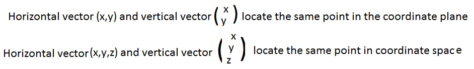
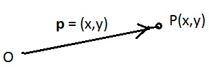
The arrays like (x,y) and (x,y,z) located points in the coordinate plane and space. In previous volume, each point P had a position vector OP = p from the origin to the point. It will not create any confusion to allow the array to denote the position vector as well as the point. Therefore, the linear combination of points
Many of the definitions and theorems in this chapter concern the coordinate plane. But often they may be extended to similar definitions and theorems involving coordinate space, often simply by extended the array from two to three numbers. For each statement that can be extended, before it will be a superscript sp3 or sp3. The first means that there is an obvious exctension to space. The second is colored, and it serves as a link. Click on it to go to where the extension is displayed or discussed. For example P(x,y)sp3 means P(x,y,z). Without arrays point P and position vector p may be in the plane or space, unless surrounding discussion or information indicates which.
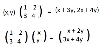
Traditionally, vertical vectors are used. But in these discussions horizontal vectors appear. (To convert to traditional notation, apply the transpose operation to the matrix and the horizontal vector.) If M is the matrix in the first equation of (*) above, then that first equation may be written horizontally as
Calculate the matrix product of (5,-1)M, or
Use the formula; substitute 5 for x and -1 for y in both expressions x + 3 and 2x + 4y
If only the latter is used to find what points are carried onto what points
[1.1]sp3 (Linear transformation on the plane)
Let α and β represent any real numbers. The expression αx + βy is called a linear expression in x and y
A linear transformation L on the coordinate plane has its formula defined by linear expressions in x and y:
(**)
Examples of different linear transformations L on the coordinate plane are:
L(x,y) = (5x - 7y, 2x + 8y),
L(x,y)=(x,0),
L(x,y) = (y,x),
L(x,y) = (x cos 45° + y sin 45°, -x sin 45° + y cos 45°)
The idea of a function carring a point onto another point is expressed by saying the function moves that point. But if the function carries the point back onto itself the function is said to leave the point fixed. The following is an identifying characteristic of linear transformations.
[1.2] Every linear transformation leaves the origin fixed.
Notationsp3: L(0,0) = (0,0).
The proof is trivial. In definition (**) above, replace x and y by 0. Then
L(0,0) = (α10 + β10, α20 + β20) = (0,0).
An important role for [1.2] is to single out and identify transformations on the coordinate plane, that are not linear. The transformation T on the coordinate plane defined by
[1.3] sp3 (Associated linear transformations and matrices) A linear transformation L on the coordinate plane and a 2x2 matrix M are associated if and only if L(x,y) = (x,y)M.
Intuitively speaking, a linear transformation is associated with a matrix if they do the same thing with each point in the plane.
The geometric nature of many linear transformations on the coordinate plane are of interest. For example, some of the linear transformations to be discussed rotate figures about the origin. Others reflect figures across a line through the origin. Both do their actions without distorting the figures; the figures and their images are congruent. These geometric properties for the linear transformations translate into algebraic properties for their associated matrices. The computer can be used to tell if a linear transformation has a certain geometric property by examining the associated matrix for the corresponding algebraic property. This is especially useful for linear transformations on coodrinate space, where the computations with matrices may be tedious.
Since arrays are 1x2 matrices they may be added and multiplied by a real number λ:
(a) (x1, y1) + (x2, y2) = (x1 + x2, y1 + y2);
(b) λ(x,y) = (λx, λy)
A linear transformation L "preserves" addition of arrays and multiplication by a real number to produce the following theorem:
[1.4]sp3 (Properties of any linear transformation on the coordinate plane) Let L be any linear transformation on the coordinate plane, let (x,y), (x1, y1), (x2, y2) be any points in that plane and let λ be any real number. Then L satisfies the following two conditions:
(a) L( (x1, y1) +(x2, y2) ) =
L(x1, y1) + L(x2, y2).
(b) L( λ(x,y) ) = λL(x,y).
In words, L carries the sum of two points onto the sum of their images. L carries the product of a real number and a point onto the product of that real number and the image of the point.
Click here to see a proof of [1.4]
The following is the traditional definition of a linear transformation. In it points (x,y), (x1, y1) and (x2, y2) have been replaced by their position vectors v,u,v respectively.
[1.5] (Defining properties of a linear transformation) A function L on a vector space is a linear transformation if and only if it has the following two properties, for all elements u and v in the vector space, and any real number λ:
(a) L(u + v) = L(u) + L(v);
(b) L(λv) = λL(v)
Notice that [1.5a] makes a linear transformation also an additive homomorphism.
Definition [1.1] is a particular case of [1.5] because [1.5] includes linear transformations on spaces very different from the coordinate plane and coordinate space. Click here to see an example of such a linear transformation. Elementary calculus is involved.
The expression
For simple geometric interpretations of [1.5a] and [1.5b] click here.
The following are applications of [1.5]:
[1.6] (Linear transformation and linear combinations) Linear transformations carry linear combinations onto linear combinations, but leaving the real number coefficients unchanged.
Notation: For any position vectors a,b,c,d and any real numbers α, β, γ, δ and any linear transformation L:
(i) L(αa + βb) = αL(a) + βL(b);
(ii) L(αa + βb + γc) = αL(a) + βL(b) + γL(c);
(iii) L(αa + βb + γc + δd) = αL(a) + βL(b) + γL(c) + δL(δd);
Intuitively speaking, in going from the left side of each equation to the right side, the linear transformation passes over the coefficients and affects only the vectors.
These examples are easily extended to linear combinations with more than four vectors. However, in this volume, such linear combinations are seldom needed.
Proof of (i):
L(αa + βb) = L(αa) + L(βb) = αL(a) + βL(b) using [1.5a] and then [1.5b]
sp3The special points (1,0) and (0,1) deserve attention. They have been given names E1 and E2 so that they have point vectors e1= (1,0) and e2= (0,1) locating those points. (Often names i and j are used instead of e1 and e2 to avoid subscripts.) Their importance is due to the facts that
[1.7]sp3 (Images of the special points determine a linear transformation) Let L and L' be two linear transformations on the coordinate plane. If L(1,0)=L'(1,0) and L(0,1)=L'(0,1) then L=L' (everywhere).
For any point (x,y), L(x,y) = xL(1,0) + yL(0,1) = xL'(1,0) + yL'(0,1) = L'(x,y).
Intuitively speaking, [1.7] says that its images of the special points completely determine a linear transformation. The following statement tells what happens if both images are the origin.
[1.8]sp3 (The zero linear transformation) A linear transformation on the coordinate plane carries all points onto the origin if and only if it carries both special points (1,0) and (0,1) onto the origin (0,0).
Notation: L(x,y) = (0,0) if and only if both L(1,0) = (0,0) and L(0,1) = (0,0).
If L carries all points onto the origin, then it carries both special points onto the origin.
Conversely,
if both L(1,0)=(0,0) and L(0,1)=(0,0) then for any point (x,y),
A linear transformation on the coordinate plane carries points onto points, and therefore carries an entire geometric figure in the plane onto something. An important question about the transformation, "does the linear transformation distort the figure?" "Does the 'something' look like the original figure?"
The most simple of all geometric figures that is not just a point is a line segment. Given a line segment with end-points A,B, where A and B are distinct points. If L is the zero linear transformation given in [1.8] then L carries the entire segment onto a single point (origin). The transformation distorts the figure. Therefore, the transformation is not being sought.
Any linear transformations that does not distort figures cannot carry any segment with distinct end-points onto a single point. Restated without a double negative: being sought are linear transformations that carry distinct points onto distinct points, that is, linear transformations that are one-to-one functions.
[1.9]sp3 (Linear transformations that carry distinct points onto distinct points) A linear transformation with a non-singular associated matrix carries distinct points onto distinct points.
Click here to see the proof.
Let a linear transformation be singular or non-singular if and only if the associated matrix is singular or non-singular. Then [1.9] can be stated: A non-singular linear transformation carries distinct points onto distinct points.