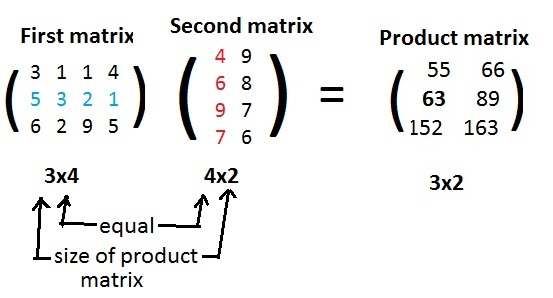
The sizes of the two matrices are important because they determine if the matrices can be multiplied together (conformable for multiplication). The following matrices ready for multiplication have sizes 3x4 and 4x2 in that order:
[1.1] (Multiplication of matrices)
(a) A first matrix is conformal with a second matrix for multiplication if the number of entries in each row of the first matrix equals the number of entries in each column of the second matrix.
(b) The dot product of the entries in row I in the first matrix with the entries in column J of the second matrix produces the entry in row I and column J in the product matrix.
Since much computation may be involved, the computer may be used to calculate the product of two conformable matrices. Click on Computer (MatProduct) to go to the program. The reader might well use the computer to verify the above matrix multiplication.
Given in (#) matrices A and B and their product AB and their reverse product BA (the reader may verify the products):
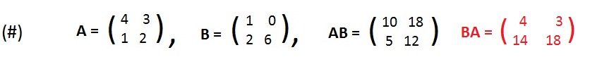
Although computing the matrix products and the determinant values of square matrices is considerable there is a simple relationship between determinants and matrix multiplication. To see an example of this relationship, compute separately and individually the determinant values of (black) matrices A, B, AB in (#) above:
[1.2] (Determinants of products of matrices) The determinant value of the product of two square matrices of the same size is equal to the product of the determinant values of the two matrices.
Notation: det (AB) = (det A)(det B), where A,B are both square matrices of the same size.
This theorem makes det a homomorphism from the collection of all the square matrices of the same size into the real number system: det preserves multiplications.
Click here for a proof of [1.2] for 2x2 matrices and their determinant values. A similar proof for 3x3 matrices is not given (very much computation). The proofs for square matrices of any size are done differently and are beyond the scope of these discussions.
Click Computer (DetProduct) to run a computer program that accepts entries from the reader for two square matrices of the same size and with integer entries, forms their product and determinants and shows each time a verification of [1.2].
An important consequence of [1.2] is the following:
[1.3] (Products of non-singular square matrices) The product of any two non-singular matrices of the same size is a non-singular matrix of that size.
The proof is trivial. If det(A) ≠ 0 and det(B) ≠ 0 then det(AB) ≠ 0. because the real number system has no divisors of zero. The properties of our common number systems affect the structures of more abstract algebraic systems such as matrices.
Non-singular square matrices play an important role in this section. Let GMatn be the collection of all non-singular matrices of size nxn. The discussions below involve matrices in GMat2 and GMat3. However, they are true for GMatn for any natural number n.
After a new operation has been defined on some objects, it may be important to see if any collections of those objects form groups. In a multiplicative group it is possible to multiply any object with itself. This means that only square matrices can be objects in a multiplicative group. The collection of all 2x2 and 3x3 matrices will be investigated here. The theorems about them will also apply to larger square matrices, but proofs given here involving the smaller matrices may or may not serve as proofs involving larger matrices.
[1.4] The collection GMatn of all non-singular nxn matrices is a multiplicatived group.
[1.4a]: closure of GMatn Closure of GMatn under matrix multiplication is a restatement of [1.3].
[1.4b]: associativity of GMatn The product operation on non-singular 2x2 matrices and on non-singular 3x3 matrices is associative.
Notation: A(BC) = (AB)C, for all square matrices A,B,C of the same size.
This property will be assumed true and no proof is given here.
Recall that the number 1 (the multiplicative identity) has the special property that 1x = x and x1 = x for any number x. In other words, multiplication of 1 with any number returns that same number. The two matrices
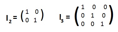
[1.4c]: identity matrices in GMatn There exists a 2x2 identity matrix I2 such that for any 2x2 matrix M: MI2 = M and I2M=M. There exists a 3x3 identity matrix I3 such that for any 3x3 matrix M: MI3 = M and I3M = M.
The reader can easily verify the four matrix multiplications with identity matrices:
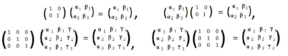
It is customary to omit the subscripts 2 and 3 on I. Seldom will this cause confusion. Therefore, the figure shows IM=I and MI=I for two different sizes of matrices.
In the common number system the numbers 2, 6, -4 have multiplicative inverses 1/2, 1/6, -1/4 because

[1.4d]: inverses exist Each matrix in GMatn has an inverse.
Notation: M-1 denotes the inverse of a matrix M. By definition (M)(M-1) = I and
(M-1)(M) = I.
The number 0 (zero) has no multiplicative inverse. For any number x, 0⋅x = 0. Therefore, no product of 0 with any number x will equal 1. A similar situation happens with matrices. If a square matrix M is singular (det M = 0) then the matrix product MY of M with any matrix Y will be singular (see [1.2]). But the Identity matrix I is non-singular, det(I) = 1.
Given a square matrix M, how to find its inverse M-1? But before any attempt to find the inverse, see if M is non-singular. If det (M) =0, then it is a waste of time to try to find M-1, it does not exist. If M is non-singular then there is a method using simple algebra (but it may be computational) to compute the inverse. Click here to see this method in action.
The computer may be used to find the inverse of a matrix, if it exists. It does not exist if the matrix is not square or is singular. Otherwise the computer first computes the adjoint of the given matrix. (The reader may go online and ask Google about adjoint. No explanation is given in this discussion about how the adjoint is computed, except to say that it always is the same size as the given matrix.) Intuitively speaking, the adjoint is "almost" the inverse matrix. The computer also computes the determinant value of the given matrix. If it is not zero then the computer will say, "divide the determinant value into the adjoint matrix to produce the inverse matrix."
Click Computer (MatInverse) to get the program. As an example, input on the keyboard the entries of the black 2x2 matrix above. The computer should produce the equivalent of the red matrix. In this case, the determinant value of the given matrix is 1, so the adjoint matrix is also the inverse matrix.
To solve for the unknown number x in the equation