In these discussions the the concept of a matrix may be considered an extension of the vector-array of numbers introduced in the previous volume. There the algebraic properties of arrays were discussed first and then geometric applications were introduced. The algebraic nature of matrices are discussed first below after Section 1. Some geometric applications will be given in a later chapter.
In this volume the assistance of the computer is used. Click on Computer (name) to go to a page where programs can be run. Then click on the name of the program for computer action.
			Jim	Sally	Rich	Frances
	T		Bob	Jack	Rose	Violet
			Joseph	Bill	Ann	June
The table has size 3 rows and 4 columns which is written 3x4. All tables are rectangular. The table has a name T. The names of the people are called entries of the table.
Sometimes natural numbers are supplied to indicate the row numbers and column numbers, but they are not part of the table. They are used in pairs to locate any entry.
	 		   1	   2	   3	   4

		 1	Jim	Sally	Rich	Frances
	T	 2	Bob	Jack	Rose	Violet
		 3	Joseph	Bill	Ann	June
The notation [2,4] denotes a location of an entry in some table, namely in row 2 and in column 4. Then this fact can be written:
Consider the following table S as another class in another room with chairs arranged the same way, 3 rows with 4 chairs in each row. In this class the following people occupy the chairs:
			John	Steve	Ed	Florence
	S		Nancy	Agnes	Lilly	Jack
			Quincy	Vance	Peter	Lem
Then table S has the same size 3x4 as table T. Also also true is the following:
The following is an important yet natural defintion:
[1.1] (Equal tables) Two tables are said to be equal if and only if:
(a) they have the same size;
(b) all pairs of corresponding entries are equal.
If R is the table
			John	Steve	Ed	Florence
	R		Nancy	Agnes	Lilly	Jack
			Quincy	Vance	Peter	Lem
then R = S.
Notice that the equality between R and S means the equality between 3x4=12 corresponding entries.
But if Q is the table
			John	Steve	Ed	Florence
	Q		Nancy	Donna	Lilly	Jack
			Quincy	Vance	Peter	Carol
			Quincy	Vance	Peter	Caro
	W		Nancy	Donna	Lilly	Jack
			John	Steve	Ed	Florence
The notation
			John	Florence   Ed	Steve
	X		Nancy	Jack	Lilly	Donna
			Quincy	Carol	Peter	Vance
If the number of rows in a table is equal to the number of columns then the table is said to be square. For example, the table
			Sally	Rich	Frances
	P		Jack	Rose	Violet
			Bill	Ann	June
is square because number of rows and the number of columns are both 3. For square tables it is possible to interchange rows and columns: row 1 becomes column 1, row 2 becomes column 2, and row 3 becomes column 3. This type of interchange is called a transposition. The transposition of table P is
			Sally	Jack	Bill
	P'		Rich	Rose	Ann
			Frances	Violet	June
Table P' is called the transpose of table P.
Notice that the operation of transposition does not move the entries Sally, Rose, June. Imagine a diagonal line is drawn through the three entries. The three entries are said to lie on the main diagonal of the table P. The three entries Frances, Rose, Bill lie on the secondary diagonal of table P.
 If all the entries in a table are numbers then the table has many mathematical properties. Some of which will be discussed in the remainder of this volume. A matrix is a table in which all entries are numbers. Most often the numbers will be integers but fractions and decimals may be in some matrices.
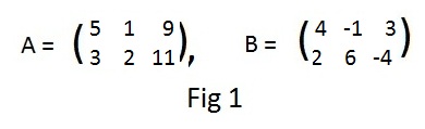
Consider the following three sets of linear equations in two unknowns:
5x + y = 9		5u + v = 9		5α + β = 9				A
3x + 2y = 11		3u + 2v = 11		3α + 2β = 11
Matrix A contains the same essential information from each set of equations. Intuitively speaking it is a abbreviated form of the equations; what is done to the equations may be done to the rows of matrix A. For example, during the process of solving the equations, for each set multiply the top equation by 2 and subtract the bottom equation from the result. A similar operation may be done on the rows of matrix A. The solutions to the equations are:
x = 1			u = 1			α = 1
y = 4			v = 4			β = 4
The three pairs of equations are the same except for the letters. So are the three pairs of solutions. These facts indicate that the letters play a minor role. Click here for an optional discussion of using just the rows of the matrix containing only integers to find the solution containing only integers.
The top row of matrix A forms a 1x3 matrix (5 1 9). Similarly, the matrix of row 2 is (3 2 11). These are equivalent to the vector arrays
Vector addition of vector arrays was defined in the previous volume as the addition of corresponding coordinats:
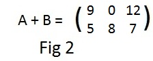
Then the sum of matrices A and B will be the matrix with row 1 = (9,0,12) and row 2 = (5,8,7), see Fig 2.
The sum of the two matrices was obtained by adding corresponding coordinates of the vectors. But those corresponding coordinates are also corresponding entries in the matrices A and B. This idea leads to the following definition, which is the first step toward making conformable matrices an additive group:
[2.1a] (Conformable matrices) Two matrices are conformable for addition if they all have exactly the same size.
[2.1b] (Addition of matrices) The sum of two matrices conformable for addition is obtained by adding corresponding entries.
Notation: If A and B denote conformable matrices then A + B denotes the matrix that is their sum.
When no confusion may arise, the phrase "for addition" in the full phrase "conformable for addition" will often be be omitted in this section. (In a later section there will be the phrase "conformable for multiplication".)
The first part [2.1a] gives the condition that matrices may be added. If the sizes are different then they cannot be combined. The second part [2.1b] tells how to add conformable matrices.
The set of all vector arrays of the same size form a commutative additive group. Using that fact with row vectors it is not difficult to prove that the set of all conformable matrices form a commutative additive group. The zero vector with all coordinates equal to zero is the additive identity for vectors. Therefore, the zero matrix 0 with all entries equal to zero is the additive identity for all conformable matrices. Here 0 denotes the zero matrices of any size. The addditive inverse of a vector array is obtained by negating all the coordinates. Then the additive inverse of a matrix is obtained by negating all of its entries.
[2.2] (Additive group of matrices) The set of all conformable matrices is a commutative additive group.
The conformable matrices with addition inherits the additive group properties directly from its numerical entries.
[2.3] (multiplication by a number) The product of a number and a matrix is (a matrix) obtained by multiplying every entry by that number.
Notation: λA where λ is any (real) number.
Unlike addition of two matrices, multiplication of a number and a matrix can always be performed. No need to talk about conformability. However, no attempt is made to define the sum of a number and a matrix (not 1x1).
If A is the matrix in Fig 1, the reader can compute A + A + A and 3A separately to obtain the same matrix.. Similarly, B + B = 2B.
There are two distributive laws:
[2.4a] (Left distributive law) For any number λ and any pair of conformable matrices A and B,
[2.4b] (Right distributive law) For any numbers λ and σ and any matrix A,
Let the reader verify that
The above statements guarantee that conformable matrices form a vector space. But this fact will not be used. Also, the dot and vector products of two matrices are not defined here, nor is the absolute value of a matrix.
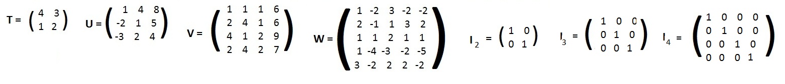
The computer assigns the determinant values 5,-42,41,118, 1,1,1 to the following matrices T,U,V,W, I2,I3,I4:
Fig 3
Click here for a discussion that shows how to obtain the determinant value by hand using a method called "cross-hatch." That method is limited to matrices with sizes 2x2 and 3x3. (There is a method called "expansion by minors" that will produce the determinant value of a 4x4 matrix using 3x3 matrices. The interested reader may go online and ask Google about the expansion.) For matrices with sizes larger than 3x3 computer must be used, and will also be used on the smaller matrices.
To call for the computer to compute the determinant value of a square matrix, click on (Computer (GetDetValue). Then click on the program GetDetValue. The program will ask where the data is located, in a file (F) or if you will type it in using the keyboard (K). Answer with K. The computer will need to know the size of the matrix: type 2x2, 3x3, 4x4 or any size les than 13x13. Then type in the entries, one at a time, followed by pressing the enter key each time. When finished the computer will output the matrix and its determinant value. When finished with the answer press enter again to remove black window. Repeated use of the same program may be done by clicking on it again. When finished with the program, click on the red rectangle with the white X in the center at the upper right of the screen. For practice use the computer to find the determinant values of matrices T,U,V,W and some of the identity matrices in Fig 3 above.
Matrices and their determinant values can be used to solve some linear equations. Given the equations:
(*)
From these three equations four 3x3 matrices are formed:
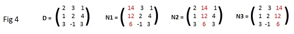
The computer assigns determinant values as follows:
The following equations have only two unknowns:
det(D) =(3)(3) - (2)(2) = 5
det(N1) = (5)(3) - (0)(2) = 15
det(N2) = (3)(0) - (2)(5) = -10.
Then
x = det(N1)/det(D) =15/5 = 3;
y = det(N2)/det(D) = -10/5 = -2.
The determinant value of a square matrix may be any number, positive or negative or even zero. If the determinant value is zero then the square matrix is called singular. Also a matrix is non-singular if the determinant value of the square matrix is not zero. In finding the values of the unknows in the above equations quotients were formed det(N1)/det(D), det(N2)/det(D) .... with the determinant value of D as the denominator in each quotient. The coefficient matrices for both systems of equations were non-singular. Therefore, solutions could be found. This discussion supports the following statement. Cramer's rule supplies a proof of it.
[3.1a] (Existence of a proper solution) If the coefficient matrix of a system of n linear equations in n unknowns is non-singular then a unique solution exists.
But if the coefficient matrix is singular then the quotients cannot be evaluated because division by zero is not allowed. The coefficient matrices of the following pairs of equations are identical and singular:
[3.1b] (No unique solution) If the coefficient matrix of a system of n linear equations in n unknowns is singular then either there is no solution or there are infinitely many solutions.
The singularity of the coefficient matrix predicts indicates that it is not worthwhile to try to solve the equations using the familiar methods. Furthermore, it is the values numerator determinants det(N1), det(N2), ... can be used to determine the number of solutions: none or many solutions.
Theorems [3.1a] and [3.1b] provide a reason for the name "determinant": it (the determinant value of the coefficient matrix) determines whether a system of linear equations may have a unique solution or not..
Recall from the last volume that u = (4,1,2) , v = (1,2,3), w=(14,7,12) may be considered as vectors in space. Using their coordinates as entries, they bcome row vectors in a 3x3 matrix
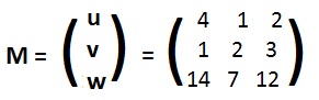
[3.2a] (Dependent rows of a matrix) A square matrix is singular if and only if its rows are linearly dependent.
This theorem says that the singularity of M guarantees the existence of numbers α, β, γ not all zero satisfying:
On the other hand the vectors computation will show that if the vectors are a = (1,4,8), b = (-2,1,5), c = (-3,2,4) then the equation
[3.2b] (Independent rows of a matrix) A square matrix is non-singular if and only if its rows are linearly independent.
The proofs of [3.2a] and [3.2b] will be discussed later:.
The determination of the singularity of a square matrix using the computer can save much work in determining the linear dependence or independence of vectors., which are also row vectors of the matrix.
Click here to see a related topic about the determinant and homogeneous equations.
There are several useful properties of determinants that are useful in various discussions. They are proven for determinants of 3x3 matrices, the proof for 2x2 matrices is almost trivial. The theorems are true for all square matrices, but proofs are not given here.
[3.3] (Transpose equal value) The determinant values of any square matrix and its transpose are equal.
![]() Let M be any 3x3 matrix and M' its transpose. See adjacent figure. The cross-hatch method produces the following expressions:
Let M be any 3x3 matrix and M' its transpose. See adjacent figure. The cross-hatch method produces the following expressions:
det(M) = aek + bfg + cdh − ceg − afh − bdk
det(M') = aek + dhc +gbf − gec − ahf − dbk
Except for the order of the products, each term in det(M) is equal to a term in det(M').
The proof for any 2x2 matrix and its transpose is even easier. The reader can produce that proof.
Based on [3.3] is the intuitive statement "what is true for rows of a matrix is also true for columns." For example
[3.4a] (Row of zeros) If every entry in a row of a square matrix is zero, then the determinant value of the matrix is zero.
[3.4b] (Column of zeros) If every entry in a column of a square matrix is zero, then the determinant value of the matrix is zero.
The point is that a proof of [3.4b] is not needed if a valid proof of [3.4a] is exists.
The cross hatch method passes diagonal lines through every row. Therefore, each product-term in computing the determinant value has a zero in it. A sum of six zeros is still zero. (For a determinant with two rows of entries, the sum of two zeros is still zero.)
However, linear dependent rows of a square matrix show that a determinant value can be zero without any zero entries in the matrix. See above.