Table of Contents /
Preface
CHAPTER 2
Section 2.1 Introduction to Trees
Of the different ways to look at a graph there is the global view - a look at the graph as a whole, and seeing all of the nodes and all of the edges or arcs. A local view sees one or a few nodes and all of the edges or arcs that touch those nodes, temporarily ignoring the rest of the graph.
For example a map of roads connecting several towns gives a driver of a car a global view of the region. WIthout a map another driver enters one of those towns and sees a junction of several roads leading out of that town. He reads a sign listing the neighboring towns and makes a decision which road to use. He has a local view of the region.
Determining the degree of a node comes from a local examination. The number of all the nodes in a graph requires a global examination..
A global view of a drawing of a ugraph can show if the ugraph is connected, if there is only one component. A local view of a node may show that node, all of its neighbors and edges touching the node.
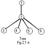 A global view also reveals any loops. It is an easy task to draw a ugraph without loops. Fig 2.1a shows such a ugraph. It has the appearance of an upside-down tree (or bush), where the root is above the branches. This is a customary way of drawing a tree - upside down, with the branches slanting downward..
A tree is a connected ugraph without any loops. Usually a single node of such a ugraph is given the distinction of being the root of the tree. In Fig 2.1a node 1 is the root.
It is obvious from the drawing that for any node (not the root) there is a path connecting that node and the root. For each node there is only one connecting path.
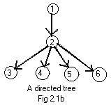 Motion entering at the root can go down to any node in a tree, making a unique directed path to the node. Fig 2.1b shows a digraph. It is a special digraph. In it every node has a single arrow pointed to it, except the root. The root has no arrow pointing to it. Sometimes an arrow is drawn to the root from the " outside" to indicate that the entry point into the graph for motion is the root.
A directed tree is a digraph in which every node is the head of a single arc, except for the root. The root is the only node that is not a head of any arc.
Each node in a digraph can be examined locally to see if it satisfies the definition of a directed tree. If each arc in a directed tree is replaced by an edge then the resulting ugraph is a tree. Compare Fig 2.1b and Fig 2.1a. That the definition of a directed tree is strong enough to imply connectivity of the entire underlying ugraph is discussed in additional material.
Often the discussion of a directed tree is more simple than the discussion of a (undirected) tree, but in many text books on graph theory it is customary to consider only trees. But at the root node all arrows point away from it (node 1), so the root node can be drawn anywhere, and the arrows need not point downward. This display of directed trees happens in the next sections.
If motion starts with the root and goes down far enough it will end up at anode from which there is no continuing path. This happens in both Fig 2.1a and Fig 2.1b. The nodes 3,4,5,6 stop further motion, they are dead ends.
In a directed tree the nodes that are heads and not nodes are called leaves. (They have arrows pointing to them, but not from them. In an undirected tree a leaf has degree 1 (only one edge touches it). The root is not included in this definition unless the root is the only node in the tree.
It is easy to draw a ugraph without loops, even if the ugraph is NOT connected. So there are more than one component. But each component is connected and cannot have loops. Therefore each component is a tree.
A forest is a ugraph without any loops.
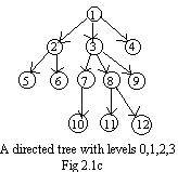 In Fig 2.1c is a larger directed tree. For it the adjacency array is:
1,2,3,4, 2,5,6, 3,7,8,9, 4,0, 5,0, 6,0, 7,10, 8,11,12, 9,0, 10,0, 11,0, 12,0 //
The zeros are optional, but they mark clearly the leaves.
Every node number appears as a leading integer in bold. Except for the root number, every node number appears once and only onceas a secondary integer (not bold or zero). This is characteristic for a labeled directed tree. These integer labels are on those nodes which have arrows pointing at them.
There is an important characteristic of a directed tree. To any node there is a directed path from the root to that node. Because there are no loops there is only one such path. There is a unique number of arcs in that directed path. The level of any node is the graphical length of the directed path to that node (i.e. the number of arcs in that directed path). In Fig 2.1c the nodes 2,3,4 are at level one, the nodes 5,6,7,8,9 are at level two The nodes 10,11,12 are at level 3. The root will always be at level zero.
There is a simillar discussion for undirected trees.
Notice how the integer labels have been assigned to the tree in Fig 2.1c. The head of each arc has a label larger than the tail. (The arrow goes from a smaller integer to a larger integer.) On any level the integer to the right is one more than the integer to the left. The integer to the extreme left at any level is one more than the integer at the extreme right in the previous level. Also the integers 1,2,...12 has been assigned to all twelve nodes This will be called in these notes the natural assignment of integer labels to a tree.
A tree is a very important idea in Graph Theory and in various parts of applied mathematics. More discussions of trees are given in the next sections and in a later chapter.
From this section 2.1 goto: additional material / problems / computer programs /
facts and theorems
===================
Section 2.2 Spanning Tree 1
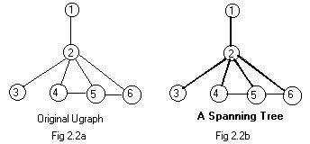 Fig 2.2a is a global view of a connected ugraph. In the figure suppose that the nodes represent six towns, and the edges represent electrical power lines between them. A power generating station (not shown) gives power to town 1, an entry point for electrical power. Then all of the towns receive electrical power through the various lines. Actually this ugraph is the original plan of the wiring before construction.
But some of the power lines are not needed. Electrical power can still reach all six towns even if lines 4-5 and 5-6 are never included in the final plan. The resulting figure is shown in Fig 2.1a. It is no coincidence that the exclusion of the two edges also prevents all loops in Fig 2.2a from forming. Yet all the nodes stay connected after the omissions. Line 2-3 cannot be omitted, because node 3 would not be connected any more. Town 3 would not receive any electrical power.
The process here is to omit as many edges as possible yet all the nodes remain connected.
Yet it is desirable to show the original plan and what lines are omitted. This process produces a connected subgraph without loops. It has the darker edges in Fig 2.2b. The lines to be omitted are shown with lighter edges.
Notice that the (dark) subgraph is a tree because there are no dark loops. Also all nodes in the original ugraph are part of the darker subgraph.
A spanning tree is a special subgraph of a ugraph. The subgraph is itself a tree and the subgraph contains all of the nodes of the original ugraph.
A different spanning tree for the original ugraph in FIg 2.2a can be found by omitting different edges of the loops. For example, include all edges (and nodes) of the original ugraph except edges 2-5 and 2-6.
A spanning tree cannot exist if the original ugraph is not connected. (But each component may have its own spanning tree.)
From this section 2.2 goto: additional material / problems / computer programs /
facts and theorems
===================
Section 2.3 Spanning Tree 2
In the previous section a spanning tree was obtained by excluding some edges of loops. This requires a global view of the entire original ugraph. Therefore a computer program for this process may be difficult to write. In this section a spanning tree will be discovered by "building up" the ugraph from scratch.
Assume that the nodes are already given. One by one each edge is to be attached to the two nodes that will be its two end points. The process will show if an edge can be excluded (drawn as a thin light edge) from the subgraph (drawn with heavy dark edges).. Otherwise the edge becomes part (made dark) of the subgraph. In any case each edge becomes part of the original ugraph.
Atention is focused on the components that are created. Before any edges are added, each isolated node is a component. As edges are added (A) the number of components may decrease, or(B) they may stay the same.
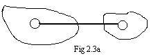 (A) If the edge being added has its end points in different components (see Fig 2.3a) then the edge becomes a "bridge" between those two components. Then they are no longer separate components. They become one bigger component. The number of components decreases by one.
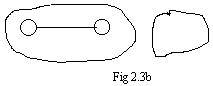 (B) If the edge being added has both its end points in the same component (see Fig 2.3b) then there is no change in the number of components. However, this happens only if the added edge completes a loop in that component. The addition of edges will not remove any loops. Therefore this loop will appear in the final (original) ugraph, after all of the edges have been added.
Recall a notation for a component containing labeled nodes. If nodes X,Y,Z are in the same component, then Y and Z are in (component) [X]. For brevity the component notation will use the color red and omit the brackets [ ]. That X,Y,Z are in component with X can be written briefly as a horizontal table
X Y Z
X X X
The black letters are integer labels of nodes They are in the components directly below them.
In the process of adding edges it will be important that all of the (black) node integers in the same component be over the same component integer. To make it more definite, the largest integer label on any node in each component will denote a component. For example, in fig 2.3c the four components are 7,9,10,11. The following table shows in what component each node is located:
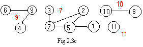
node 1 2 3 4 5 6 7 8 9 10 11
comp 7 7 7 9 7 9 7 10 9 10 11
The ugraph in Fig 2.2a has edges 1-2, 2-3, 2-4, 2-5, 2-6, 4-5, 5-6. Ignoring these edges the ugraph becomes a collection of descrete nodes 1,2,3,4,5,6. Each node then is a whole component by itself. The table for this is
node 1 2 3 4 5 6
comp 1 2 3 4 5 6
If the first edge 1-2 is added then a new component is created by merging the two discrete components 1 2. Then node1 and node2 are in the same component and 2 is the larger integer. The revised table is:
node 1 2 3 4 5 6
comp 2 2 3 4 5 6
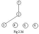 Addition of the next edge 2-3 enlarges the component containing node1 and node2 to a new component that contains node1, node2 and node3 (see Fig 2.3d)
node 1 2 3 4 5 6
comp 3 3 3 4 5 6
Addition of edges 2-4, 2-5 and 2-6 enlarges this same component:
node 1 2 3 4 5 6
comp 4 4 4 4 5 6
node 1 2 3 4 5 6
comp 5 5 5 5 5 6
node 1 2 3 4 5 6
comp 6 6 6 6 6 6
This last table shows that all nodes are in the same component as node6. The ugraph is connected. This is the table for the tree shown in Fig 2.1a.
It is interesting to see what happens to the last table when the next edge 4-5 is added to the ugraph. NOTHING. And for the addition of edge 5-6 again nothing. The component [6] is not enlarged because the table remains the same. The additions of these last two edges produce loops. In a drawing these two edges should be drawn lightly. The other edges are darker and show a spanning tree. See Fig 2.2b.
It is important to know that the whole process of adding edges and determining what edges make loops does not require a drawing. This means that the process can be done by a computer. More information about this process can be found in additional material .
From this section 2.3 goto: additional material / problems / computer programs /
facts and theorems
===================
Section 2.4 Spanning Tree 3
In this section a third and final method for deriving a spanning tree is described. Motion is used in much the same way that in a psychology laboratory a rat moves in a maze of corridors and rooms. However, the motion will be more systematic, and not so random. But since motion is involved, this method requires a local view of each node.
In a house of rooms and corridors linking the rooms, there is important evidence in each room. But much time is required to uncover and examine the evidence in each room. A detective is given the task to examine the evidence in all of the rooms. Naturally he does not want to examine the same room twice. After he finishes his examination of a room, he leaves a marker, say a bright yellow piece of paper. If he sees the marker in a room, he will not go forward into that room.
One room has a door to the outside. The detective enters the house through that door into the start room. He will visit and examine all of the rooms, and then returns to leave by that same door. Suppose Fig 2.2a represents the plan of rooms and corridors. He enters at room 1 and examines the evidence there.
He leaves a marker in room 1 and goes forward along the corridor to room 2 and examines the evidence there. He leaves a marker in room 2. Now he must make a choice because there are four corridors leading from room 2 to rooms without yellow markers. Say he chooses the corridor to room 3. He goes foreard to room 3, examines the evicence there and leaves a marker.
But now he is stuck in room 3. He cannot go forward out of that room to another room that does not have a marker. He backs up from room 3 back to room 2. He does not examine the evidence in room 2. Instead he chooses to go along anonther corridor, say to room 4. He examines the evidence there and leaves a marker.
He can go forward out of room 4 to room 5. (For this method of moving about the house the detective prefers to go forward if he can, not backward. See additional material for more information about this preference.) In room 5 the detective examines the evidence and leaves a marker.
Following his preference he goes foreward to room 6. There he examines the evidence and leaves a marker.
Since he can go no further forward, he backs up back to room 5. (He always backs up to a room that he has just left previously.) In room 5 he can only back up to room4. He backs out of room 4 to room 2. (He does not back up to room 3 because he entered room 4 from room 2, not from room 3.) He backs up out of room 2 to room 1. He can leave the house now by backing through the door to the outside.
 If the detective has the plan of the house, namely the rooms and corridors, he can retain a diary of his movements with arrows along the edges representing corridors. If he traverses a corridor he draws an arrow from the node of the room that he has just left to the node of the room that he has entered. (He could paint an arrow along the corridor itself, but the owner of the house would object.) When the detective backs out of a room to a previous room he is going against the direction of the arrow joining those two rooms.The arrow from node 1 to node 2 made previously tells the detective to back up from 2 to 1, and not from 2 to 3.
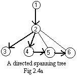
The drawing of arrows produces a directed tree as shown in Fig 2.4a. The dark portion fulfills the conditions of a directed tree. Also it spans the original ugraph in Fig 2.2a because its arrows point to all of the nodes (except the root). Iit is another directed spanning tree of the same ugraph and is different from that shown in Fig 2.1b.
At this time the question of which directed spanning tree is "better" is not being considered.
From this section 2.4 goto: additional material / problems / computer programs /
facts and theorems
Table of Contents /
Preface