 They are represented on paper as two small separated circles called nodes or vertices in Fig 1.1a. The node to the left represents the water tower. (Imagine that we are looking down on the two objects.)
There are already many excellent textbooks on Graph Theory. They discuss the many topics in that field. These notes do not contribute new topics to that field, but rather give more detailed discussion to the introductory topics and in a more intuitive way. The basic idea is to make progress in smaller steps, appealing to intution and to use of simple examples from everyday life.
Many peope with inquisitive minds, especially those with scientific interests, will ask what various things have in common. For example, what do the following systems have in common: a system of roads in a state, a maze, a grid of power lines, a system of pipes supplying water to a city, a bond of atoms in a complex organic molecule etc? Extraction of the common properties from these systems leads to the idea of a graph. It can be drawn on paper or created as data in a computer to represent any of these systems.
Strictly speaking a graph is special type of drawing, often on paper. But often it represents some physical situation, like a map, plan or blueprint. In section 1.2 parts of graphs receive numerical labels and a horizontal notation is developed for labeled graphs. In section 1.3 there is a discussion about two graphs being equivalent.
This chapter, chapter 1, introduces some basic ideas of graphs, such as digraphs, ugraphs, labeled graphs and equivalent graphs. But discussions beyond these topics will begin in Chapter 2.
On a separate pages are discussions about theorems and more formal facts about graph theory.
Exercises help persons to understand the discussions and executable computer programs are available by download to expand interest and to avoid some computational drudgery. For these programs use a PC with a Windows or DOS operating system. A special directory must be created. At the top level of the C: root directory create the directory GRAPHTH.
Click on the word in hypertext in these notes to receive (additional) directions, information or material.
Also needed are some "tools" from Windows.
A list of executable programs accompanies these notes.
A graph is a crude mode or outline of a collection of objects linked togethertogether. In representing such a physical situation the graph usually includes only a few details taken from the situation. In most cases graph theory discussed here is not sensitive to color, shape, or texture of individual objects. To what graph theory is sensitive is one of the tasks of these notes.
The following shows how three very simple objects linked together are represented by drawn graphs. They illustrate their fundamental building blocks.
(A) A new house is built. A water tower already stands not far away.
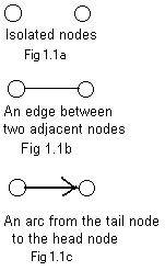
They are represented on paper as two small separated circles called nodes or vertices in Fig 1.1a. The node to the left represents the water tower. (Imagine that we are looking down on the two objects.)
(B) The house needs a supply of water. A ditch is dug (or a pipe is laid) and links the two objects. See Fig 1.1b. In the drawing a line segment, called an edge, links the two nodes. (A bent line or simple curve can also be used as a drawn link.) Two nodes with an edge between them are said to be adjacent or neighbors. The two nodes are called end points of the edge. An edge touches (technically is incident with) a node if the node is an end point of the edge. By its definition a single edge never can touch three separate nodes or just one node. It must have exactly one node at each end of it (end points).
(C) Water flows through along the bed of the ditch. See Fig 1.1c It flows from the tower on the left to the house on the right. In the drawing an arrow called an arc (or directed eddge), indicates the direction of the flow. It goes from the one node, called the tail, (in this situation the tower) to the other node, called the head (the house). Intuitively speaking, the arrow is drawn over the link in Fig 1.1b, like the water flowing on and over the ditch. If the flow of water is stopped, then the ditch is empty and can be represented by an edge. In some future discussions arcs may sometimes be replaced by the edges beneath them.
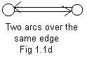 In the early chapters of these notes two nodes may be linked by one edge, but not by more than one edge. However, there may be two arcs going in opposite directions as shown in Fig 1.1d. Think of this drawing as representing a single two lane road between two cities, but motion of vehicles in each lane goes in opposite directions. Therefore only one edge lies beneath a pair of arcs going in opposite directions.
Over an edge there are four possibilities: no arc (just an uncovered edge), one arc, an arc going in the other direction, or a pair of arcs going in the opposite directions.
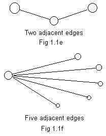
The idea of adjacency can be applied to edges. Adjacent edges have a common end point. They touch the same node. Fig 1.1e shows two adjacent edges. The common node in the middle has two nodes adjacent to it. Each of the edges "touches"the common node.
In Fig 1.1f there is a generalization. There are 5 adjacent edges. The common node at the left has 5 nodes (neighbors) adjacent to it. The 5 nodes form a neighborhood of the common node but not of each other (no links).
The degree of a node is the number of edges touching it. It equals the number of nodes in its neighborhood. An isolated node has degree zero. The degree of the common node in Fig 1.1e is 2, and the degree of the common node in Fig 1.1f is 5.
Up to this point the discussions involved basic parts of graphs. By themselves they form trivial graphs, but do not form big enough graphs with enough parts to become anything interesting. The following identify structures of all shapes and sizes.
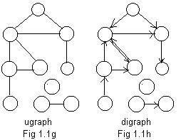 A graph is a finite collection of nodes and any links between pairs of those nodes. If the links are edges as in Fig 1.1g then the graph is called a ugraph for "undirected graph." If the links are arcs (as in Fig 1.1h) then the graph is a digraph for "directed graph." "Under" each digraph is a ugraph, which can be revealed by removing or replacing the arcs (arrows) by edges (line segments). In Fig 1.1g the ugraph exists by itself. But "under" the digraph in Fig 1.1h is a ugraph identical to the ugraph in Fig 1.1g.
The Fig 1.1g shows a single ugraph, even though there are three "pieces" in the ugraph. For example it might be a road map for ten towns on three islands. On the big island are seven towns. On another island are two towns, and on the third small island just one town where no cars are allowed.
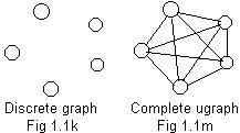
For any finite collection of nodes there are two extremes concerning edges linking pairs of those nodes. Examples are shown in Fig 1.1k and Fig 1.1m for five nodes. The graph in Fig 1.1k has no links. Every node is isolated in a discrete graph. Such a graph is not very interesting.
The ugraph in Fig 1.1m is saturated with edges, No more edges are possible. In a complete ugraph all pairs of nodes are linked.
The prefix sub- is often used to mean "a part of." For example, a subcommittee is part of an original committee, which is usually bigger than the subcommittee. As far as members of the bigger committee, some members are included in the subcommittee, while some are not. But the subcommittee retains the quality of a genuine committee in itself.
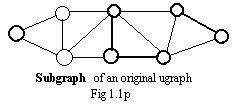 Sometimes attention is focused on a part of a graph, which will be called the original graph. The part contains none, some or all of the nodes of the original graph, but no node outside of the original graph. All included are none, some or all of the edges or arcs of the original graph. If an arc is included in the part, then the end points (nodes) of the arc must be included. Then the part is called a subgraph of the original graph
In Fig 1.1p the subgraph has 3 darkened edges and 6 darkened nodes. It is part of the entire figure which is the original ugraph. The subgraph is a graph by itself, but is contained in the larger original graph.
The idea of a subgraph is quite general. A single node is considered a subgraph. Also all the nodes without edges or arcs form a subgraph. Both subgraphs are trivial, uninteresting and discrete. For technical reasons it is convenient to allow an empty graph with no nodes or links, and the entire original graph to be subgraphs.
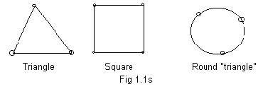 The geometric figures of triangle, square, rectangle, hexagon are polygons with closed perimeters. See Fig 1.1s. A perimeter goes around and meets itself. The perimeter forms a loop. A loop can be made from a single piece of rope by tying its ends together. The ugraphs in Fig 1.1g and Fig 1.1p have two loops each, all triangular. In Fig 1.1m there are many loops, some with 3 edges, some with 4 edges and one with 5 edges. A loop in a ugraph must have 3 or more edges. The role of loops and a more detailed description of them will be given in subsequent sections.
All graphs discussed in this work are finite. This means that no graph can have an infinite number of nodes, nor an infinite number of edges or arcs.
The drawings in the above discussions show graphs consisting of nodes and links. They show the basic structures of graphs, nothing more. In future sections of these notes information and labels will often be assigned to nodes and/or links of basic structures.
From this section 1.1 goto: additional material / problems / computer programs / facts and theorems
==============================
In the previous section a drawing is used to represent a graph. Usually the basic structures are better understood in a drawing. Many ideas in graph theory are discussed accompanied by such drawings.
However, along with discussions in this work there will be computer programs to help process data from graphs. The drawings themselves do not serve well as data for computers programs. Moreover, occasionally it will be necessary to focus attention locally on some node in a graph. Assign a label (name) to that node to avoid confusion with any other node. Do this with all the nodes in the graph. WIth most situations the reader or author may assign these names, usually in the form of integers. Modern computer languages can and do assign integer labels to nodes of graphs that have been somehow represented in memory (through the use of pointers serving as arcs of the graph).
In these notes only positive integers will be assigned to nodes. These integer labels do not change in any way the basic structures of the graphs, no more than a room number on the outside of a door changes what is inside a hotel room.
There are many ways to select the integer labels from all the integers, but two rules of assignment will always be followed:
(1) no single integer will be assigned to two different nodes in the same graph,
(2) no integer less than 1 will be assigned to any node.
Some authors include programs written in the C or C++ languages. They find it convenient to allow zero as an integer label because of the structure of arrays in those languages. However zero and also negative integers will be used for other purposes in programs that accompany discussions in this work; they should not be used as integer labels on any nodes.
Because all graphs under discussion are finite, the number of nodes is finite. While counting all the nodes it may be convenient to assign integers 1,2,3,... as labels. (However other positive integers could be used.)
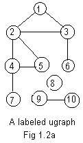 For example, the nodes in Fig 1.1g have received integer labels 1,2,3,4,5,6,7,8,9,10 as shown in Fig 1.2a. The same ten integers could be assigned to the ten nodes in some different arrangement, but the basic structure remains unchanged.
The links do not need labels, because they can be identified by the labels on the end points (nodes). Placing a hyphen between the labels on end points, all of the edges in Fig 1.2a are
# 4-7, 6-3, 10-9, 1-3, 2-1, 5-2, 4-5, 3-2.This horizontal list has several defects. First, its lack of order makes it difficult to use as data for human use. Second, it does not involve the isolated vertex 8. It is not a complete arithmetical description of the ugraph.
The (full) adjacency array is a more convenient and compact way of writing an arithmetical description of a labeled ugraph. It is not difficult to write this array down from a drawing. In Fig 1.2a the smallest integer is 1. It has neighbors 2 and 3. Then form a cluster of integers 1,2,3. Form a second cluster starting with 2. That cluster is 2,1,3,4,5. The next cluster is 3,1,2,6. The last cluster from the drawing is 10,9. In each cluster the first integer is called the leading integer. The remaining integers in a cluster follow the leading integer and are called secondary integers.
The clusters are conveniently displayed as a horizontal array in which the clusters are separated by one or more spaces:
U 1,2,3, 2,1,3,4,5, 3,1,2,6, 4,2,5,7, 5,2,3,4, 6,3, 7,4, 8, 9,10, 10,9//The spaces between clusters are necessary. They make the reading the array easier. More importantly, the spaces avoid confusing leading integers with the secondary integers of the previous cluster. (The single slash / can also be used as separators of clusters.) The double slash // at the end of the array is used to indicate end of the array. The U is a reminder that the adjacency array after it is for a ugraph. It is not part of the adjacency array. It does not correspond to anything in the drawing. The spaces and slashes are important as delimiters for data imput to a computer.
It is optional, but a zero may be placed after the 8 to indicate that 8 is a label on an isolated node. The zero is not a true label, because zero cannot be assigned to any node. Yet 8,0, looks more like a cluster than does 8, .alone by itself.
In each cluster of the full adjacency array, the number of positive secondary integers is equal to the degree of the node to which the leading integer is assigned. For example the cluster 4,2,5,7 has three secondary integers 2,5,7. The node 4 has degree three. In the cluster 8,0, there are no positive secondary integers. Therefore node 8 must have degree zero.
Using the leading integer repeatedly with each secondary integer in each cluster a horizontal list of (genuine) edges appears from the full adjacency array:
1-2 1-3 2-1 2-3 2-4 2-5 3-1 3-2 3-6 4-2 4-5 4-7 5-2 5-4 6-3 7-4 9-10 10-9These can be rearranged:
1-2 2-1 1-3 3-1 2-3 3-2 2-4 4-2 2-5 5-2 3-6 6-3 4-5 5-4 4-7 7-4 9-10 10-9This last listing shows that each edge is listed twice. It is possible to delete repetitions so that a shorter list will show all the edges once and only once. To avoid complexity we will use the full adjacency array U just discussed. See additional material for a discussion of full (U) and short adjacency arrays.
A second and slightly different type of array is the digraph(D).
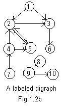 There is a similar hyphen notation for the arcs in a labeled digraph in Fig 1.2b which has the basic structure as the digraph in Fig 1.1h..
1->2 1->3 2->3 2->5 3->6 4->2 4->5 5->2
7->4 8->0 9->108->0 is a pseudo-arc. For digraphs it is sometimes useful to indicate nodes that are "dead-ends" like nodes 6 and 10. They are not tails. There are no arcs going out of them, so if motion is involved no exit is possible from them. The notation 6->0 and 10->0 may be included in the above arrow notation, even though they are not isolated nodes.. This is the first hint that digraphs may be more difficult to handle than ugraphs.
The adjacency array for the digraph in Fig 1.2b is
(D) 1,2,3, 2,5, 3,6, 4,2,5, 5,2//In any single graph to be labeled never will the same integer-label be assigned to two different nodes. In some situations the lowest integer, might indicate by default a "start" or "entry" place to start an examination or to process the graph. In these notes no node will receive zero label nor any negative number. The adjacency arrays must involve all nodes and edges or arcs of the graph to be a complete description of that graph. Pseudo-links should be used for all isolated nodes.
It is fairly easy to look at a drawing of a graph and write down the adjacency array. But it can be very difficult to draw a graph from a long adjacency array. Yet the array, properly written, contains a complete determination of the basic structure of a graph, as far as our study of graph theory is concerned. Some developments later in these notes will give some help in drawing a graph from the arrays.
For this section 1.2:
Additional material /
Facts and Statements /
Problems /
Programs
==============================
Although it is not generally observed in many conversations in English, there is a difference in the meanings of the words "equal" and "equivalent" used in these notes The equation A = B means that A and B are really (denoting) the same object. It is true if A=5 and B=5 in algebra. It is true if person A and person B are the same person. If a person has two names, say "Jim" and "John", then Jim = John.
But if Jim and John are two different people, but are capable of doing the same job effectively and completely, then as far as the job is concerned Jim and John are equivalent. It can be written Jim ~ John.
Intuitively speaking, two objects are equivalent (object1 ~ object2) if most of their distinguisting properties are ignored. By agreement a few properties are used to decide their equivalence or non-equivalence.
This idea of equivalence can be applied to graphs. The basic structures of two or more ugraphs are equivalent (more commonly called isomorphic) if they cannot be distinguished from one another from the point of view of graph theory. A more precise definition is given in additional material .
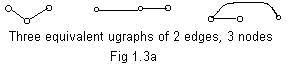 Two edges are equivalent, even if they are drawn with different lengths, colors, either edge is bent. The three ugraphs in Fig 1.3a are created by linking a node to two other nodes with edges. The equivalence can also be seen by a special assignment of integer labels to the nodes, and looking at the adjacency array. Assign 2 to the node of degree 2 (the node that is joined to the other two nodes). Assign 1 and 3 to the remaining nodes. For each of the ugraphs the adjacency array is the same (equal):
It is important to know that the nodes must be assigned labels in a special way to two equivalent graphs to get identical adjacency arrays. But unlike adjacency arrays for two graphs prove nothing.
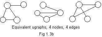 The basic structures of three equivalent ugraphs are shown in Fig 1.3b. Three nodes and edges form a loop (triangle) and an edge sticks out from one of the vertices of the loop. It is not important here that in the ugraph on the right two edges are drawn crossing each other because their intersection is not a node.
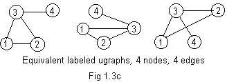 In the labeled ugraphs of Fig 1.3c the integer label 3 has been
assigned to the node that has three edges touching it. Labels 1 and 2 are given to the other two nodes of the loop (triangle). 4 is assigned to the other end of the edge sticking out from the loop. All three ugraphs have the same adjacency array, namely:
In the labeled ugraphs of Fig 1.3c the integer label 3 has been
assigned to the node that has three edges touching it. Labels 1 and 2 are given to the other two nodes of the loop (triangle). 4 is assigned to the other end of the edge sticking out from the loop. All three ugraphs have the same adjacency array, namely:
Using the same integer label for nodes in different ugraphs somehow relates the nodes. That assignment makes the nodes correspond. The same integer (3) was assigned to the nodes in the different ugraphs to those nodes of degree three. And the same integer (4) was assigned to nodes of degree one. The other two nodes in each ugraph may be assigned the remaining integers (1 and 2) in either order. In this way a complete correspondence between all the nodes of the different ugraphs is constructed. Actually the correspondence could be constructed without the use of integer labels, but it is much more convennient to use them. Different colors and shapes of nodes could be used.
The following assumption is made without proof: If all the nodes in two ugraphs are assigned integer labels so that their individual (full) adjacency arrays are identical, then the basic structures of those two ugraphs are equivalent (isomorphic). A similar assumption can be made about digraphs.
Often it may be possible to show non-equivalence of two ugraphs by visual inspection of their basic structures. Upon comparing the ugraphs certain conditions may be found that prevent equivalence. Many of these conditions may be deduced from the above assumption.
Any one of the following conditions guarantees that two graphs under comparison are NOT equivalent:
[A] They have a different number of nodes.
[B] They have a different number of isolated nodes (one has possibly zero number of isolated nodes).
[C] They have a different number of edges.
[D] They have a different number of loops.
[E] If one ugraph is (totally) connected and the other ugraph is not connected (has more than one piece).
[F] For all the nodes of degree k in either ugraph, then there is a different number of nodes of degree k in the other ugraph. Allow k to be zero (see condition B) or any positive integer.
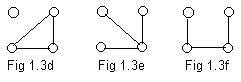 The ugraphs shown in Fig 1.3d, Fig 1.3e, Fig 1.3f are not equivalent basic structures because of the conditions listed above. Only the ugraph in Fig 1.3d has a loop. By condition [D] it is not equivalent to the other ugraphs. In Fig 1.3e a node has degree 3. None of the other two ugraphs have a node of degree 3. So the ugraph in Fig 1.3e is not equivalent to either of the other two, by condition [F].
It would be a waste of effort to assign integer labels 1,2,3,4 in different orders to each of the three basic structures and try to get identical adjacency arrays. But a computer program could direct a computer to carry out an exhaustive procedure of assignments of labels, and show that the adjacency arrays are always different. That would also show that the ugraphs are not equivalent. Again a waste of time.
In many situations of comparing two ugraphs it may be difficult to find any application of rules A-F. Again resort to the computer. The method of blindly assigning different integer labels to the basic structures of two ugraphs has the nature of "brute force." It requires testing possibilities, usually many, to discover one equivalence, or testing all possibilities to show non-equivalence. Using the brute force method for two graphs each having 13 nodes, more than 6 billion calculations may be needed to prove that they are not equivalent. Considerable time on a desk top or laptop computer would be needed..
This leaves open the general problem of deciding if the basic structures of any two ugraphs are equivalent or not, where the number of nodes is the same, and the number of edges is the same, and those numbers are large.
For this section 1.3:
Additional material /
Facts and Statements /
Problems /
Programs
==============================
 It is very useful to extend the ideas of an edge and an arc. They allow motion to go from one node to a second adjacent node. After arriving at the second node motion may continue and go to a third node, which is adjacent to the second node. This motion may continue going from a node to an adjacent node a finite number of times. All this takes place in some graph.
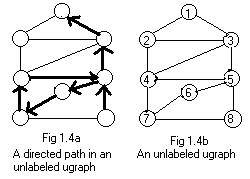
In Fig 1.4a is a sequence of 7 arrows indicating motion starting from the node on the lower right going to the top node. Each arrow indicates a motion from one node to an adjacent node.
In Fig 1.4b there are no such arrows. Since the graph is labeled the sequencecan be indicated by a chain of integers:
8 -> 5 -> 6 -> 7 -> 4 -> 5 -> 3 -> 1
The arrows in Fig 1.4a and the chain of integers denote a directed path from one node to another distant node. The lower right node (8) is the tail or start node of the directed path, and the top node (1) is the head or end node.
Another directed path can be made from start node 7 to end node 5 (see Fig 1.4b):
7 -> 4 -> 3 -> 1 -> 4 -> 5
The directed paths are composed of arcs, but the arcs lie over edges. These edges form an undirected path between two nodes.
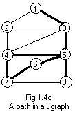 Motion may go in either direction along an undirected path, so there are no start or end nodes, just end points of the undirected path. Nodes 1 and 8 are end points of an undirected path in Fig 1.4c.
In most works on Graph Theory the term path means undirected path. A path is a generalization of an edge, which has no direction. In Fig 1.4c there is a path between node 1 and node 8. The same path is also between 8 and 1. The chain of integers for this path is:
8 - 5 - 6 - 7 - 4 - 5 - 3 - 1
This is the same path as:
1 - 3 - 5 - 4 - 7 - 6 - 5 - 8
A path containing several nodes is like a (one lane) road without any traffic but with several towns on the road. There is no motion, just a way to go.
A path contains any finite number of edges. (Similarly a directed path contains any finite number of arcs.) That number is called the graphical length of a path (or of a directed path). The term "graphical" is used to distinguish this length from a sum of physical lengths or values that can be assigned to each edge or arc. In Fig 1.4c the graphical length of the path between node 1 and node 8 is seven. It is equal to the number of dashes in the chain of integers that represents the path.
It will be convenient to have paths of graphical length zero. Actually it is a theoretical path that goes from any node back to the same node with no other nodes involved.
If motion goes from one end point of a path to the other end point then motion traverses the path. If motion traverses the path in Fig 1.4c then it produces a directed path as in Fig 1.4a (or a directed path in the opposite direction).
The edges in a path and the arcs in a directed path are joined together end for end. There is no break or interruption in a path; it is continuous between the end points. This fact suggests the following definition.
 Two nodes in a graph are connected if there is a path between them. It will later be convenient to say that any node is connected to itself, even though there may not be an actual path from the node back to itself.
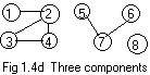
In Fig 1.4d node 1 and node 4 are connected, because path 1 - 2 - 4 connects them. (Is there another path connecting nodes 1 and 4?) Node 6 and node 7 are connected. Node 8 is connected to node 8. But node 2 and node 5 are NOT connected because there is no path between them. In Fig 1.4b every node and node 5 are connected.
There is a very suggestive notation that can be introduced here, even though it is not used in other works on Graph Theory. Let X denote the integer label on any node. Let [X] denote all the nodes connected to node X. Include in [X] all the edges (from the ugraph) that link the nodes in [X]. (Thus [X] is a subgraph of the original graph.) Then [1] = the left piece (subgraph) of the graph in Fig 1.4d. [5] = middle piece (subgraph), and [8] = the one piece (subgraph) that has only node 8 in it.
Since node 2 is connected with nodes 1,2,3,4, [2] = [1]. In fact [1] = [2] = [3] = [4]. They all denote the same subgraph. Also [5] = [6] = [7]. [8] is equal only to itself.
A component containing node X is that subgraph, in which all nodes are connected to X. From the original graph include all edges that link these nodes. In a drawing the component appears as the largest subgraph in one piece containing node X.
The idea of components breaks a ugraph down into whole pieces. Inside each piece every node is connected to every node. Each component is isolated because it cannot have a connection (path) with any other component. In Fig 1.4d there are three components.
A physical example is a county of several islands with no bridges. On each island are roads linking towns. Then a road map of the county is a ugraph containing several components. The county could build enough bridges so that the former components are linked and become one big component.
It is also true that two graphs each with a different number of components cannot be equivalent. Moreover, equivalent graphs must have equivalent components. The county road map changes if bridges are built linking some of the islands or if new roads are built on some island.
An entire graph is connected if every node in it is connected to every node in it. Clearly a connected graph has just one component, namely itself. In Fig 1.4a the (entire) graph is connected. Connected graphs have certain useful properties. A component of any graph will also have these properties.
Some paths are special; not every graph has them.
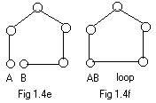 Fig 1.4e shows a path as defined above. It has two end points A and B. Now stretch the bottom edge so that B moves to the left and eventually coincides with A. See Fig 1.4f. This is also considered a path. By borrowing a term from handling ropes the following definition is produced:
A loop is a path with coincident end points. All other nodes in a loop are distinct. A more common and more technical definition of a loop is given in additional material . In many text books on graph theory a loop is called a cycle or a circuit.
In Fig 1.4c there is a loop 5-6-7-4-5. In the chain notation for a loop one (or more) of the node numbers must be repeated. Here 5 is repeated. Intuitively speaking, node 5 is actually two coincident end points of the path that forms a loop to the left of node 5. Motion to traverse the loop begins and ends there.
Experiment will show that a loop must have at least 3 edges and at least 3 nodes so that the loop does not collapse into two coincident edges. The "smallest" loops have the shapes equivalent to triangles.
Loops occur naturally in graphs. And they may be part of paths, as shown in FIg 1.4c. In traversing the path from node 8 to node 1 motion traverses extra edges unnecessarily when it goes around the loop starting at 5. Also motion could traverse the loop many times. (This might happen to a person lost in a maze of corridors.) The idea here is that loops can produce undesirable results when working with graphs.
Two graphs each with a different number of loops cannot be equivalent.
Some paths have loops in them, and some paths do not. A path is simple if it has no loops. A simple path extends the idea of an edge. The path in Fig 1.4e is simple. In Fig 1.4c the path 8-5-3-1 is simple. In a simple path no node is included twice. Therefore, in the chain of integers for a simple path no integer appears more than once. Intuitively speaking, motion going along a simple path will NOT meet any fork in the path (like going up the stem of the letter Y).
There are graphs in which every path is simple. Some of these important graphs (trees) will be discussed in Chapter 2.
A simple path is a special kind of path. More paths with special properties are discussed in additional material including directed loops and simple directed paths. Also there are brief discussions of paths called Eulerian and Hamiltonian.
For this section 1.4:
Additional material /
Facts and Statements /
Problems /
Programs