Again it can be said that the material presented in this volume is not that of a detailed text book. It presents some ideas informally and does not justify some procedures completely. However, it does allow the reader to experience those procedures by the input of data and execution of programs. The programs serve another purpose. They free the reader from long, tedious and time-consuming computations. Therefore references to computer usage appear often, and require some ability to use a computer. The recent versions of the Windows operating system and Windows Explorer are recommended for readinig these web pages.
Try the same procedure with
But a link is of two types:
(A1) an undirected line (or curve) that shows no direction while joining two nodes
(A2) a directed line (or curve) like a vector symbol that points from one node to some other node.
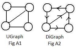
Fig A1 shows a graph of four nodes with undirected links (also called edges). Such a graph is called a Ugraph. Among other representations, Ugraphs represent things listed in (a1) above.
Fig A2 shows a graph with the same four nodes, but with directed links (also called arcs). That graph is a Digraph. Digraphs can be used to represent things listed in (a2) above. In this chapter and in the next all links are undirected. In chapter 3 Digraphs will be discussed.
An abbreviation is used for the type of graph, U for a Ugraph, and D for a Digraph.
The examples in (a1) and (a2) suggest that motion can be used to distinguish directed and undirected links. Along an undirected link, motion is allowed in either direction (like a two-lane road), but along a directed link motion is allowed only in one direction (like a one-way one-lane road). The motion may be animated by the movement of a bug or particle going along a link between two nodes.
A pair of linked nodes are two distinct nodes with a link joining them. In Fig A1 the diagonal makes the upper-right and lower-nodes linked nodes. WIthout another diagonal the nodes upper-left and lower-right are not linked nodes.
There are many kinds of Ugraphs. In this volume, only those Ugraphs that satisfy the following conditions will be discussed.
[1.1](Restrictions on links and nodes) In any collection of all links and nodes:
(a) only a finite number of nodes are involved; (Usually the number is small.)
(b) a link joins exactly two distinct nodes
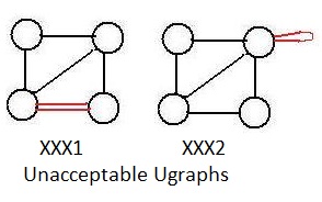
(c) never more than one (undirectional) link connects two nodes. (Violation shown in XXX1)
Condition (b) implies that no link can join any node with itself. (Violation shown in XXX2).
It also implies that a single link cannot pass through a third node. It is true that there is a "path" between the node in the upper-left and the node in the lower-right in Fig A1 going through another node, but it is not a link.
 To show a violation of (b) in the drawing XXX2, the offending link has been bent. But acceptable bent links between nodes will appear in later drawings.
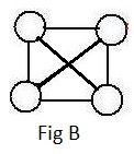
Links that even cross each other are acceptable (Fig B). Again [1.1b] prevents their point of intersection to be a node.
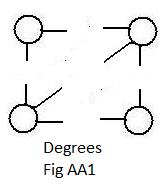
The basic structure of a Ugraph are the nodes and links. The basic structure is determined by every node and its links with other nodes. Those other nodes are called its neighbors. In Fig A1 the upper-left node has two neighbors, but the lower left node has three neighbors. It is easier to count neighbors by counting links contacting a node. Figure AA1 is an exploded view of Fig A1 in which the links are cut making it is easier to count the number contacts. The number of links contacting a node (equal to the number of neighbors) is called the degree of that node. The nodes on the upper-left and lower-left of the graph have degree 2 and 3 respectively.. But the nodes on the upper-right and lower-right have only degree 3 and 2 respectively.
It is usually easy to determine the degree of each node in a Ugraph. In some larger graphs it may be difficult to count all the many links. The following fact is then helpful.
[1.2] The sum of the degrees of all the nodes in a Ugraph is equal to twice the number of all the links.
When the degrees are determined for two nodes at the ends of the same link, that link is counted in each degree, therefore it is counted twice. This happens for all the links. Therefore, the sum of all the degrees will be twice the number of links. Is [1.2] true for discrete graphs? (In a discrete graph every node is isolated.)
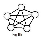
The graph in Fig B above with four nodes has a peculiar property: every pair of nodes is linked together. In the adjacent Fig BB there are five nodes and every pair of nodes are linked together. It is theoretically possible to construct a Ugraph of any number of nodes and link every pair of nodes together. After constructing all those links, no more links can be created because of [1.1b]. Intuitively speaking, the graph is "saturated" with links. A graph in which every pair of nodes is linked together is called a complete graph. A complete graph has a maximum number of links. Click here to see the discussion supporting the following statement:
[1.3] (Maximum number of links) The maximum number of links in a Ugraph with exactly n nodes is given by the formula n(n-1)/2..
If n=4 then the formula gives 12/2 = 6. That is the number of links in the complete graph of Fig B. If n=5 then the formula gives 20/2 = 10, the number of links in the complete graph of Fig BB. A graph with exactly 6 nodes cannot have more than 30/2 = 15 links.
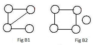
It is possible that a node have less than two links contacting it. If it has degree 1 then it is often called a leaf (see above the B1 in the adjacent FIg B1). If it has no links contacting it then it is called isolated (See above B2 in Fig B2). Isolated nodes are seldom included in discussions in this volume. However, both B1 and B2 are acceptable as Ugraphs.
The graph in Fig B above has six links. They can be counted directly, or the degrees of the four nodes can be added to give 12. Half of that is six. But that graph is "saturated with links. No more links could exist between nodes because of [1.1c]. If a graph has exactly five nodes, then ten links saturate it. A Ugraph with a maximum number of links is called a complete graph. Click here for a discussion of complete Ugraphs. There are not many interesting real life situations represented by complete graphs. The other extreme is a discrete graph. All of its nodes are isolated. No links are part of the graph. It is almost never interesting.
A complete graph is extreme; it has the maximum number of links. The other extreme is a discrete graph. It has no links. Every node is isolated. Interesting graphs usually are not extreme, neither complete nor discrete.
Labeling convention In a graph of n nodes, assign all of the natural numbers 1,2,....,n in Nn to all the nodes in a graph so that each node has a different natural number.
Notice that the convention is actually the process of counting all of the nodes.
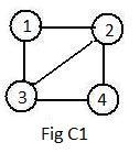
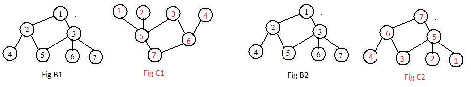
Fig C1 shows one way (actually, there are 24=4! ways) of assigning labels to the four nodes in the unlabeled graph A1. The four nodes may be represented as
After labels have been assigned to all the nodes of a graph, an array of degrees of all nodes can be determined from the drawing. For C1, the array is
A different use of parentheses and numbers provides a method of representing nodes and their neighbors. Linked nodes are called adjacent. In the graph C1, nodes 2 and 3 are its linked neighbors of 1. In this volume the following notation says the same thing:
The short adjacency list does not require that all neighbors of each node be given, only those with higher numbers:
(***)
(1),2,3,
(2),3,4,
(3),4,
(4),
The graph C1 shows that node (3) has neighbors 1 and 2. Since they are less than (3) they are not included in the short adjacency list. The node (4) does have neighbors 2 and 3, so it is not isolated as it may appear. The advantage of the short list is that less numbers are required, and yet it will define the graph for the computer. It simply converts the short adjacency list into something equivalent to the long adjacency list which has all the neighbors.
The defining information of a graph in this volume F to be given to the computer has a specific form, called input-data of the graph. For graph C1 it is:
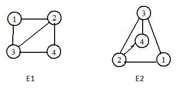 Consider the drawings in the adjacent picture. The two graphs appear to be very different. Yet the long adjacency arrays for them are identical, namely,
(1),2,3, (2),1,3,4, (3),1,2,4, (4),2,3
Their short adjacency arrays
(1),2,3, (2),3,4, (3),4, (4)
must also be identical.
[1.2] (Label equivalence) Two labeled graphs are label equivalent if and only if their short adjacency arrays are identical.
It is possible that two drawn graphs are congruent: they can be made to coincide. If one graph is labeled then it easy to copy the labels on nodes of the labeled graph onto corresponding (coincident) nodes of the other graph. The two graphs are then label equivalent.
If one graph has more nodes than another graph, then they cannot be label equivalent. If one graph has more links then more neighbors are involved. Such graphs cannot be label equivalent.
It is not difficult to show that the relation "label equivalent" satisfies the three conditions for equivalence relation. And , intuitively speaking", the computer cannot distinguish the label equivalent graphs one from the other. More about equivalent graphs will be discussed in a later chapter.
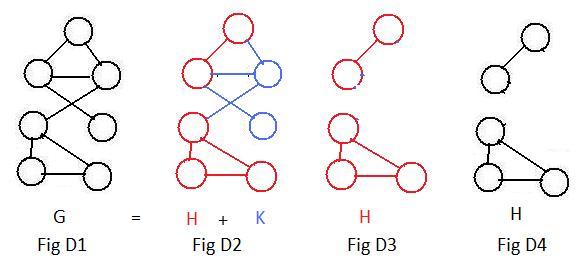
[1.3] (Subgraphs) A subgraph H of a graph G satisfies the following conditions:
(a) H itself has all of the properties of a graph according to [1.1];
(b) all of the nodes and links in H are nodes and links of G;
(c) no link in G joins a node in H with a node not in H.
Notice that the blue pieces K in Fig D2 do not form a subgraph of G because any of the blue links joins a blue node in K to a red node not in K. That violates condition [1.3c].
In Fig D3 the subgraph H has been extracted from graph G by removing all pieces K not in H. Fig D4 shows the H as genuine a graph as G but smaller. It also shows that a subgraph may have more pieces than the supergraph from which it is taken.
If nodes are removed from a labeled graph then the labels on the remaining nodes will be missing some natural numbers.
For node 1 in Fig C1, the following statements have truth values 1 or 0:
1 is a neighbor of 1 0
2 is a neighbor of 1 1
3 is a neighbor of 1 1
4 is a neighbor of 1 0
where 1 means TRUE and 0 means FALSE.
These four statements are condensed and become the row containng 1 in the following table:
     1   2   3   4
 1   0   1   1   0
 2   1   0   1   1
 3   1   1   0   1
 4   0   1   1   0
The row containing 2 means that the neighbors of 2 are 1,3,4 because 1 is under each of these numbers.
These rows are equivalent to the clusters
(1)2,3,
(2)1,3,4,
(3)1,2,4,
(4)2,3
which form the long adjacency array for graph C1.
The red matrix is symmetric about the main diagonal of all zeros because links are undirected: if x is linked to y then y is linked to x. The red table is called the adjacency matrix for graph in Fig C1.
In general, if a graph has n nodes then its adjacency matrix will be a square symmetric matrix of size nxn. But as input-data for a graph into a computer, it is large, tedious and prone to errors to prepare before input, e.g. a misplaced 1 or 0 may happen.
The graph C2 has the same adjacency matrix. Two labeled graphs are label equivalent if and only if their adjacency matrices are identical.
Condition (b) prevents cutting a link. Not allowed is a node and part of its attached link be in a subgraph and the remaining part and node be outside the subgraph. However, the link can be excluded from the subgroup, while an end node or both may be in the subgraph.
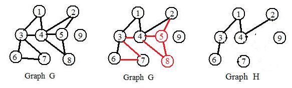
In the adjacent Fig E is a graph G, another graph G and a graph H. Some of the links and nodes in the second graph became red. They are to be removed to produce graph H. Then H is a subgraph of G. The construction of H (by partial distruction of G?) introduced no other node or link outside G into H.
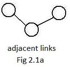 In the previous section was the definition, two nodes are adjacent if they have a common link between them. A similar definition for adjacent links is, two links are adjacent if they contact the same node. Fig 2.1a shows two adjacent links. (More links can be adjacent with a common node.) Adjacent links allow motion to go along one link, pass through the common node and then go along the other link. Motion can go in the reverse direction from a second link to a first adjacent link. In this sense adjacent links are extensions of single links.
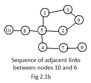 Very useful in graph theory are sequences of adjacent links. Fig 2.1b is an example of a sequence (sometimes called a walk) between nodes 10 and 6. Between those two nodes is a sequence of links each one adjacent to a previous link (except for the link in 10 - 8) and adjacent to the next link (except for the link in 7 - 6). Such sequences have a special name.
[2.1] (Paths) A path in a graph is a subgraph that is a sequence of adjacent links and nodes with degrees not exceeding 2. Two nodes are allowed to have degree 1, but it is possible that all nodes in the path have degree 2.
The sequence
Except for nodes 10 and 6, all nodes in the path have degree 2. They are called interior nodes of the path. Nodes 10 and 6 are exterior nodes or end nodes. The path connects the end nodes 10 and 6. (Actually, the path connects all nodes in the path, by creating by deletion a sub-path with any pair of nodes there becoming ends.) This word "connects" is justified by the fact that every path is continuous - there are no missing links anywhere along it.
In Fig 2.1b there is a less complicated path connecting nodes 10 and 6: 10 - 8 - 5 - 4 - 7 - 6.
All of its nodes are different; no node appears twice.
[2.2] (Simple paths) A path is simple if all its nodes are different.
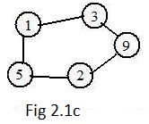 It is quite possible that a simple path connect a node to itself. In Fig 2.1c the path
[2.3] (Loops) A loop is a simple path connecting some node to itself.
In some other text books loops are called cycles.
As a subgraph, in a loop all nodes have degree 2. There are no end nodes. Since the loop is simple, no node is repeated. This presents a problem: how to denote a loop in a discussion where information is given horizontally. It is like trying to force a circle into becoming a straight line. In a horizontal sequence of labels denoting a loop, the first and last labels are the same:
In a drawing a path connecting two distinct nodes is simple if and only if it contains no loops. Such a path cannot cross itself. The path connecting nodes 10 and 6 in Fig 2.1b is obviously not simple.
A person might drive from home to another city and return home by a different way. Then his round trip has made a loop. But the trip one way from home to the city and the return trip qualify as simple paths. In the loop of Fig 2.1c notice that sub-paths
The one-to-one correspondence f is ignoring the rest of the graphs, namely the links. The following brings links into the discussion:
[3.1] (Graphical correspondences) A one-to-one correspondence
The condition "strictly preserving neighborhoods and inversely" is equivalent to the following statement:
x-y are a linked pair in G if and only if f(x)-f(y) are a linked pair in G'. Because of this interpretation, f is said strictly to preserve links. Implied in this statement is the condition that the inverse function f-1 also strictly preserves links for graphical correspondence f.
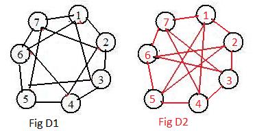 The short arrays for the graphs in D1 and D2 are
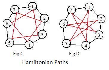
In graph D1 two loops are very obvious:
(internal) 1-3-5-7-2-4-6-1
(rim) 1-2-3-4-5-6-7.
In D2 two loops are very obvious:
(internal)1-4-7-3-6-2-5-1;
(rim) 1-2-3-4-5-6-7.
A first attempt to find a permutation that preserves links is for the function to carry rim onto rim:
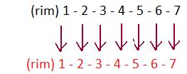
Then the function would be the identity permutation:
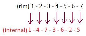
There are other permutations that carry linked nodes onto linked nodes. The computer finds all 14 permutations. They all carry the Hamiltonian rim loop of D1 onto the internal Hamiltonian loop of D2. They also carry the Hamiltonian internal loop of D1 onto the rim loop of D2.
Question: if the red numbers in the array (&) are reversed 5,2,6,..., 1 does the resulting function show equivalence of the two graphs?
In general, the question, "are two given graphs with the same number of nodes equivalent?" may be very difficult or impossible to answer in some cases, even for people with extensive knowledge of graph theory using super fast computers. Click here for a short explanation.