 They are represented on paper as two small separated circles called nodes or vertices in Fig 1.1a. The node to the left represents the water tower. (Imagine that we are looking down on the two objects.)
There are already many excellent textbooks on Graph Theory. They discuss the many topics in that field. These notes do not contribute new topics to that field, but rather give more detailed discussion to the introductory topics and in a more intuitive way. The basic idea is to make progress in smaller steps, appealing to intution and to use of simple examples from everyday life.
Many peope with inquisitive minds, especially those with scientific minds, will ask what various things have in common. For example, what do the following systems have in common: a system of roads in a state, a maze, a grid of power lines, a system of pipes supplying water to a city, a bond of atoms in a complex organic molecule etc? Extraction of the common properties from these systems leads to the idea of a graph. It can be drawn on paper or created as data in a computer to represent any of these systems.
Strictly speaking a graph is special type of drawing, often on paper. But often it represents some physical situation, like a map, plan or blueprint. In section 1.2 parts of graphs receive numerical labels and a horizontal notation is developed for labeled graphs. In section 1.3 there is a discussion about two graphs being equivalent.
This chapter, chapter 1, introduces some basic ideas of graphs, such as digraphs, ugraphs, labeled graphs and equivalent graphs. But discussions beyond these topicsl will begin in Chapter 2.
On a separate pages are discussions about theorems and more formal facts about graph theory.
Exercises help persons to understand the discussions and executable computer programs are available by download to expand interest and to avoid some computational drudgery. For these programs use a PC with a Windows or DOS operating system. A special directory must be created. At the top level of the C: root directory create the directory GRAPHTH.
Click on the word in hypertext in these notes to receive (additional) directions, information or material.
Also needed are some "tools" from Windows.
A list of executable programs accompanies these notes.
Intuitively speaking a graph is special type of drawing, often on paper or as a computer created picture on screen or in a file. But it often represents some physical situation, like a map, plan or blueprint. In a sense, the graph is a crude model of the situation by linking objects together.
In representing a physical situation the graph includes usually only a few details taken from the situation. In most cases graph theory discussed here is not sensitive to color, shape, or texture of individual objects. To what graph theory is sensitive is one of the tasks of these notes.
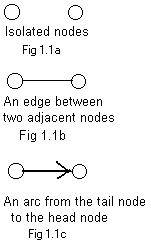
The following shows how three very simple situation are represented by drawn graphs. They illustrate the fundamental building blocks.
(A) A new house is built. A water tower already stands not far away.
They are represented on paper as two small separated circles called nodes or vertices in Fig 1.1a. The node to the left represents the water tower. (Imagine that we are looking down on the two objects.)
(B) The house needs a supply of water. A ditch is dug (or a pipe is laid) and links the two objects. See Fig 1.1b. A line segment, called an edge, links the two nodes. (A bent line or simple curve can be used as a drawn link.) Two nodes with an edge between them are said to be adjacent or neighbors. The two nodes are called end points of the edge.
(C) Water flows through along the bed of the ditch. See Fig 1.1c It flows from the tower on the left to the house on the right. In the drawing an arrow called an arc, indicates the direction of the flow. It goes from the one node, called the tail, (in this situation the tower) to the other node, called the head (the house). Intuitively speaking, the arrow is drawn over the link in Fig 1.1b, like the water flowing on and over the ditch..
The three diagrams indicate about to what in the house - water tower situation graph theory here is sensitive: two nodes, a link between them or a directed link from one to the other.
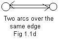 In the early chapters of these notes two nodes may be linked by one edge, but not by more than one edge. However, there may be two arcs going in opposite directions as shown in Fig 1.1d. Think of this drawing as representing a single two lane road between two cities, but motion of vehicles in each lane goes in opposite directions. Therefore only one edge lies beneath a pair of arcs going in opposite directions.
Over an edge there are four possibilities: no arc, one arc, an arc going in the other direction, or a pair of arcs going in the opposite directions.
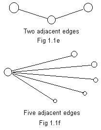
The idea of adjacency can be applied to edges. Adjacent edges have a common end point. Fig 1.1e shows two adjacent edges. The common node in the middle has two nodes adjacent to it. Each of the edges "touches"the common node.
In Fig 1.1f there is a generalization. There are 5 adjacent edges. The common node at the left has 5 nodes (neighbors) adjacent to it. They form a neighborhood of the common node.
The degree of a node is the number of edges touching it. It equals the number of nodes in its neighborhood. An isolated node has degree zero. The degree of the common node in Fig 1.1e is 2, and the degree of the common node in Fig 1.1f is 5.
Up to this point the discussions involved basic parts of graphs. By themselves they form trivial graphs, but do not form big enough graphs with enough parts to become anything interesting. The following identify structures of all shapes and sizes.
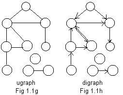 A graph is a finite collection of nodes and any links between pairs of those nodes. If the links are edges as in Fig 1.1g then the graph is called a ugraph for "undirected graph." If the links are arcs (as in Fig 1.1h) then the graph is a digraph for "directed graph." "Under" each digraph is a ugraph, which can be revealed by removing or replacing the arcs (arrows) by edges (line segments). In Fig 1.1g the ugraph exists by itself. But "under" the digraph in Fig 1.1h is a ugraph identical to the ugraph in Fig 1.1g.
The Fig 1.1g shows a single ugraph, even though there are three "pieces" in the ugraph. For example it might be a road map for ten towns on three islands. On the big island are seven towns. On another island are two towns, and on the third small island just one town where no cars are allowed.
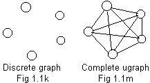
For any finite collection of nodes there are two extremes concerning edges linking pairs of those nodes. Examples are shown in Fig 1.1k and Fig 1.1m for five nodes. The graph in Fig 1.1k has no links. Every node is isolated in a discrete graph. Such a graph is not very interesting.
The ugraph in Fig 1.1m is saturated with edges, No more edges are possible. In a complete ugraph every pair of nodes are linked.
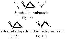 Sometimes attention is focused on part of a graph. Fig 1.1p shows a ugraph. Attention is focused on the part containing 4 nodes with darkened edges. Fig 1.1q shows an extracted copy of that part. But that part satisfies our idea of a ugraph.
We call the darkened part in Fig 1.1p a subgraph of the bigger graph in that figure. The subgraph includes some (or all) of the nodes of the bigger graph. Moreover, the subgraph also includes all of the links from the bigger graph that link nodes in the subgraph. The extracted part shown in Fig 1.1r does not include the horizontal link that joins two nodes of the subgraph. So Fig 1.1r does not represent a subgraph of the bigger graph in Fig 1.1p.
Intuitively speaking a subgraph is determined by its nodes. The links joining these nodes in the subgraph are automatically determined as part of the bigger graph. No links are added nor removed.
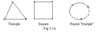 The geometric figures of triangle, square, rectangle, hexagon,... polygon have closed perimeters. See Fig 1.1s. The perimeter goes around and meets itself. The perimeter forms a loop. A loop can be made from a single piece of rope by tying its ends together. The ugraph in Fig 1.1g has two loops, both triangular. The subgraph in Fig 1.1q has one loop. In Fig 1.1m there are many loops, some with 3 edges, some with 4 edges and one with 5 edges. A loop in a ugraph must have at least 3 or more edges. The role of loops and a more detailed description of them will be given in subsequent sections.
The drawings in the above discussions show graphs consisting of nodes and links. They show the basic structures of graphs, nothing more. In future sections of these notes information and labels will often be assigned to nodes and/or links of basic structures.
For this section 1.1
Additional material
Facts and Statements
Problems
Programs
==============================
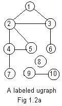 Usually the integers 1,2,3,... are assigned to the nodes. If there are N nodes then the first N positive integers are assigned to them For example, the nodes in Fig 1.1g have received integer labels 1,2,3,4,5,6,7,8,9,10 as shown in Fig 1.2a. The labels are not part of the basic structure of any graph, and can be assigned arbitrarily or by some method. However, different assignments of integers to the nodes of the same graph may affect the results of some processings of the graph.
The links do not need labels, because they can be identified by the labels on the end points (nodes). Placing a hyphen between the labels on end points, all of the edges in Fig 1.2a are
# 4-7, 6-3, 10-9, 1-3, 2-1, 5-2, 4-5, 3-2.This horizontal list has several defects. First, its lack of order makes it difficult to use as data for human use. Second, it does not involve the isolated vertex 8. It is not a complete arithmetical description of the ugraph.
The clusters are conveniently displayed as a horizontal array in which the clusters are separated by one or more spaces:
The spaces between clusters are necessary. They make the reading the array easier. More importantly, the spaces avoid confusing leading integers with the secondary integers of the previous cluster. This is important as data input to a computer.
The double zero at the end are not part of the adjacency array. They do not correspond to anything in the drawing. The zeros are used in programming to signify the end of the array to the computer.
It is optional, but a zero may be placed after the 8 to indicate that 8 is a label on an isolated node. The zero is not a true label, because zero cannot be assigned to any node. Yet 8,0, looks more like a cluster than does 8, .
In each cluster of the full adjacency array, the number of positive secondary integers is equal to the degree of the node to which the leading integer is assigned. For example the cluster 4,2,5,7 has three secondary integers 2,5,7. The node 4 has degree three. In the cluster 8,0, there are no positive integers. Therefore node 8 must have degree zero.
Using the leading integer repeatedly with each secondary integer in each cluster a horizontal list of (genuine) edges appears from the full adjacency array:
Of the two arrays for a ugraph, the full array (F) may be needed for processing correctly the data for a ugraph. But the short array (S) is easier to write down because it is shorter. It is not too difficult to convert one type of array into the other. See Additional material for discussion of the conversion.
A third type of array is the diagraph(D).
The adjacency array for the digraph in Fig 1.2b is
It is fairly easy to look at a drawing of a graph and write down the adjacency array. But it can be very difficult to draw a graph from a given horizontal sequence of many links. Yet the araray, properly written, contains a complete determination of the basic structure of a graph, as far as graph theory is concerned. Some developments later in these notes will help a little in drawing a graph from the arrays.
Although it is not generally observed in many conversations in English, there is a difference in the meanings of the words "equal" and "equivalent." The equation A = B means that A and B are really (denoting) the same object. It is true if A=5 and B=5 in algebra. It is true if person A and person B are the same person. If a person has two names, say "Jim" and "John", then Jim = John.
But if Jim and John are two different people, but are capable of doing the same job effectively and completely, then as far as the job is concerned Jim and John are equivalent. It can be written Jim ~ John.
Intuitively speaking, two objects are equivalent (object1 ~ object2) if most of their distinguisting properties are ignored. By agreement a few properties are used to decide their equivalence or non-equivalence.
This idea of equivalence can be applied to graphs. The basic structures of two or more ugraphs are equivalent (more commonly called isomorphic) if they cannot be distinguished from one another from the point of view of graph theory.
It is important to know that the nodes must be assigned labels in a special way to two equivalent graphs to get identical adjacency arrays. Unlike adjacency arrays for two graphs prove nothing.
Using the same integer label for nodes in different ugraphs somehow relates the nodes. The assignment makes the nodes correspond. The same integer (3) was assigned to the nodes in the different ugraphs to those nodes of degree three. And the same integer (4) was assigned to nodes of degree one. The other two nodes in each ugraph may be assigned the remaining integers (1 and 2) in either order. In this way a complete correspondence between all the nodes of the different ugraphs is constructed. Actually the correspondence could be constructed without the use of integer labels, but it is much more convennient to use them.
The following assumption is made without proof: If all the nodes in two ugraphs are assigned integer labels so that their individual full adjacency arrays are identical, then the basic structures of those two ugraphs are equivalent (isomorphic). A similar assumption can be made about digraphs. The word "full" should be omitted.
Often it may be possible to show non-equivalence of two ugraphs by visual inspection of their basic structures. Upon comparing the ugraphs certain conditions may be found that prevent equivalence. Many of these conditions may be deduced from the above assumption.
Any one of the following conditions guarantees that two graphs under comparison are NOT equivalent:
[A] They have a different number of nodes.
It would be a waste of effort to assign integer labels 1,2,3,4 in different orders to each of the three basic structures and try to get identical adjacency arrays. But a computer program could direct a computer to carry out an exhaustive procedure of assignments of labels, and show that the adjacency arrays are always different. That would also show that the ugraphs are not equivalent. Again a waste of effort.
In many situations of comparing two ugraphs it may be difficult to find any application of rules A-F. Again resort to the computer. The method of blindly assigning different integer labels to the basic structures of two ugraphs has the nature of "brute force." It requires testing possibilities, usually many, to discover one equivalence, or testing all possibilities to show non-equivalence. Using the brute force method for two graphs each having 13 nodes, more than 6 billion calculations may be needed to prove that they are not equivalent. Considerable time on a desk top or laptop computer would be needed..
This leaves open the general problem of deciding if the basic structures of any two ugraphs are equivalent or not, where the number of nodes is the same, and the number of edges is the same, and those numbers are large.
The full adjacency array is a more convenient and compact way of writing an arithmetical description of a labeled ugraph. It is not difficult to write this array down from a drawing. In Fig 1.2a the smallest integer is 1. It has neighbors 2 and 3. Then form a cluster of integers 1,2,3. Form a second cluster starting with 2. That cluster is 2,1,3,4,5. The next cluster is 3,1,2,6. The last cluster from the drawing is 10,9. In each cluster the first integer is called the (F) 1,2,3, 2,1,3,4,5, 3,1,2,6, 4,2,5,7, 5,2,3,4, 6,3, 7,4, 8, 9,10, 10,9, 0,0
The (F) is not part of the array. It is an optional identifier showing the type of array (full adjacency array) . The whole word (Full) could be used. There will be other arrays of different types.
1-2 1-3 2-1 2-3 2-4 2-5 3-1 3-2 3-6 4-2 4-5 4-7 5-2 5-4 6-3 7-4 9-10 10-9
These can be rearranged:
1-2 2-1 1-3 3-1 2-3 3-2 2-4 4-2 2-5 5-2 3-6 6-3 4-5 5-4 4-7 7-4 9-10 10-9
In the listing each edge is listed twice. To eliminate this double listing, delete the second edge in each pair of edges. The result is a horizontal list in which each edge is given exactly once.
1-2 1-3 2-3 2-4 2-5 3-6 4-5 4-7 9-10
For each edge x-y in this listing, the left end point x is less than the right end point y.
The array for this is
(S) 1,2,3, 2,3,4,5, 3,6, 4,5,7, 5, 6, 7, 8,0, 9,10, 10, 0,0
After 5 nothing appears because all the numbers 2,3,4 are smaller than 5. But 5 is not an isolated node. The isolated node is 8 and it is included along with a zero. It shows that node 8 is isolated. This array is called the short adjacency array (S) for a ugraph.
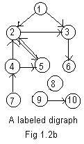 There is a similar hyphen notation for the arcs in a labeled digraph in Fig 1.2b which has the basic structure as the digraph in Fig 1.1h..
1->2 1->3 2->3 2->5 3->6 4->2 4->5 5->2
7->4 8->0 9->10 0->0
8->0 and 0->0 are pseudo-arcs. For digraphs it is sometimes useful to indicate nodes that are "dead-ends" like nodes 6 and 10. They are not tails. There are no arcs going out of them, so if motion is involved no exit is possible from them. The notation 6->0 and 10->0 may be included in the above arrow notation, even though they are not isolated nodes.. This is the first hint that digraphs may be more difficult to handle than ugraphs.
(D) 1,2,3, 2,5, 3,6, 4,2,5, 5,2, 0,0
In any single graph to be labeled never will the same integer-label be assigned to two different nodes. In come cases the number 1, or the lowest integer, might indicate by default a "start" or "entry" place to start an examination or to process the graph. In these notes no node will receive zero label nor any negative number. The adjacency arrays must involve all nodes and edges or arcs of the graph to be a complete description of tha graph. Pseudo-links should be used for all isolated nodes.
For this section 1.2
Additional material
Facts and Statements
Problems
Programs
==============================
Section 1.3 Equivalent graphs
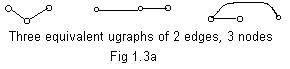 Two edges are equivalent, even if they are drawn with different lengths, colors, either edge is bent. The three ugraphs in Fig 1.3a are created by linking a node to two other nodes with edges. The equivalence can also be seen by a special assignment of integer labels to the nodes, and looking at the adjacency array. Assign 2 to the node of degree 2 (the node that is joined to the other two nodes). Assign 1 and 3 to the remaining nodes. For each of the ugraphs the adjacency array is:
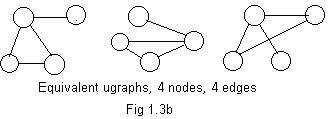 The basic structures of three equivalent ugraphs are shown in Fig 1.3b. Three nodes and edges form a loop (triangle) and an edge sticks out from one of the vertices of the loop. It is not important here that in the ugraph on the right two edges are drawn crossing each other because their intersection is not a node.
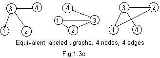 In the labeled ugraphs of Fig 1.3c the integer label 3 has been
assigned to the node that has three edges touching it.
Labels 1 and 2 are given to the other two nodes of the loop (triangle). 4 is assigned to the other end of the edge sticking out from the loop. All three ugraphs have the same adjacency array, namely:
In the labeled ugraphs of Fig 1.3c the integer label 3 has been
assigned to the node that has three edges touching it.
Labels 1 and 2 are given to the other two nodes of the loop (triangle). 4 is assigned to the other end of the edge sticking out from the loop. All three ugraphs have the same adjacency array, namely:
[B] They have a different number of isolated nodes (one has possibly zero number of isolated nodes).
[C] They have a different number of edges.
[D] They have a different number of loops.
[E] If one ugraph is (totally) connected and the other ugraph is not connected (has more than one piece).
[F] For all the nodes of degree k in either ugraph, then there is a different number of nodes of degree k in the other ugraph. Allow k to be zero (see condition B) or any positive integer.
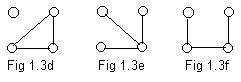 The ugraphs shown in Fig 1.3d, Fig 1.3e, Fig 1.3f are not equivalent basic structures because of the conditions listed above. Only the ugraph in Fig 1.3d has a loop. By condition [D] it is not equivalent to the other ugraphs. In Fig 1.3e a node has degree 3. None of the other two ugraphs have a node of degree 3. So the ugraph in Fig 1.3e is not equivalent to either of the other two, by condition [F].
For this section 1.3
Additional material
Facts and Statements
Problems
Programs