Go to other chapters or to other branches of math
Additional Material for this Chapter
Exercises for this Chapter
Answers to Exercises
Computer programs
Chapter 6
Geometry and Transformations
Section 1: Geometric Transformations and Universes
Again attention is focused on the four familiar geometric sets: point, line, plane and space. In discussions in this chapter some of the ideas from plane and solid geometry will be considered using some of the "tools" developed in previous chapters. Sometimes a point designated as the origin will be involved, sometimes not. In any discussion here the point, line, plane, and space will be called affine universes. The point is a trivial universe and the other three are nontrivial universes. If it contains an origin then an affine universe is also a linear universe. Discussions of geometric universes larger than space (of 3 dimensions) are beyond the scope of this chapter.
In all non-trivial affine universes the concept of parallelism exists. Planes and lines may be parallel. In these discussions they may be parallel to themselves. (This makes parallelism an equivalence relation.)
Recall that points are collinear if they lie on a common (straight) line. And they are coplanar if they lie in a common plane. Recall also that a function F carries a set S onto a set F(S) which is the totality of all points that are images of points in S. Lines and planes are sets of points. If L is a line then it is a collections of points (a subset), so that F(L) is a set (subset) of images. What F does to L geometrically is important; in other words, what is the shape of F(L) ? The function F could "bend" the line into a curve F(L) that is a parabola. In this chapter a geometric function carries any line onto a line or onto a point. This means that a geometric function carries collinear points onto collinear points. If all the images form a line, then the function is non-singular. If the function carries any entire line onto a single point then the function is singular. A geometric function carries a line segment onto a line segment (or a point).
However, the line segment and its image may or may not have the same length. A geometric function carries a plane onto a plane, or onto a line, or onto a point. In the last two situations the function is singular.
Functions that carry segments onto segments of the same length are non-singular and play a special role in geometry.
[1.1] (Distance-preserving functions) A function preserves distance if and only if the distance between any two points is the same as the distance between their images. Names for this type of function are congruence and isometry.
Notation: F preserves distance if and only if distance between any points A and B equals distance between
their images F(A) and F(B).
Example 1a:
In plane geometry two segments AB and CD are congruent if they have the same length. Using the idea just presented, there is a distance-preserving function F that carries the first segment onto the second segment such that F(A) = C and F(B) = D. The distance between A and B> must equal the distance between F(A) and F(B), which are C and D respectively.
F is not the only distance-preserving function carrying AB onto CD. Another distance-preserving function G has the property that G(A) = D and G(B) = C.
Because F and G preserve distance it can be shown that they are also one-to-one functions carrying segment AB onto segment CD.
Example 1b:
There is no reason why the two segments cannot coincide. In this situation there are two fixed points A1 and A2 and a congruent but movable X-segment on top of the A-segment. There are two ways that the X-segment can coincide with the A-segment: dont move the X-segment and pick it up flip it over and put it down on top of the A-segment. There are various ways of denoting these two events. Using the previous notation,
F(A1) = A1 and F(A2) = A2
and
G(A1) = A2 and G(A2) = A1
Using the arrow notation these two events can be described as
F: A1 --> A1 A2 --> A2
and
G: A1 --> A2 A2 --> A1
The subscripts alone can describe the two events:
1 --> 1, 2 --> 2
and
1 --> 2, 2 --> 1
But these are the two permutations of the first two natural numbers, 1,2. The idea of permutations driving the movement of a congruent figure is developed further in the next example.
Example 2:
 Let A1, A2, A3 be three fixed points that are the same distance apart in a counterclockwise direction. Then they are vertices of an equilateral triangle. On top of this A-triangle is another congruent but movable X-triangle. On top of the A-triangle the X-triangle coincides with the A-triangle. The following basic command causes what happens to X-triangle (but always all the vertices must come to rest on all the vertices of the A-triangle):
i --> j if i and j are different, move X-triangle so that its vertex above Ai is moved to a position above Aj
i --> i
do not move the vertex that is above Ai
where i and j are any of the numbers among the first three natural numbers, 1,2,3.
There are six permutations of these three natural numbers:
123, 231, 312, 132, 321, 213
(although in the previous discussions about six permutations the order was 123, 132, 213, 231, 312, 321).
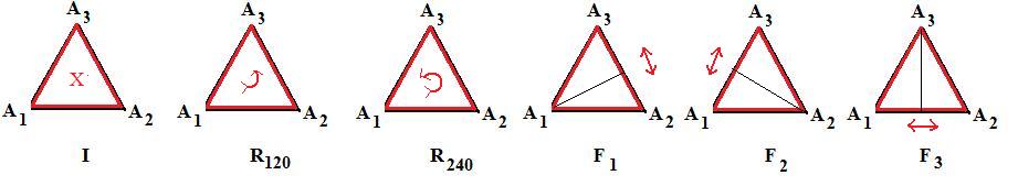
The permnutations written in full are:
[I]
1 --> 1, 2 --> 2, 3 --> 3,
[no vertices move; X-triangle does not move]
[R120]
1 --> 2, 2 --> 3, 3 --> 1,
[X-trianglerotates about its center +120°]
[R240]
1 --> 3, 2 --> 1, 3 --> 2,
[X-triangle rotates about its center +240°]
[F1]
1 --> 1, 2 --> 3, 3 --> 2,
[X-triangle is reflected about altitude from vertex A1]
[F2]
1 --> 3, 2 --> 2, 3 --> 1,
[X-triangle is reflected about altitude from vertex A2]
[F3]
1 --> 2, 2 --> 1, 3 --> 3
[X-triangle is reflected about altitude from vertex A3]
========================================
Certain conditions will be imposed on these "geometric functions" to make them "linear." The first condition is that (1) the functions always carry the origin onto the origin: F(O) = O.
If point P lies on the line through points A and B then F(P) lies on the line through F(A) and F(B). A more strict condition will be imposed. (2) F preserves ratios: ratio AP/AB = ratio F(A)F(P)/F(A)F(B), if F(A) and F(B) are distinct. For example, if P is 2/3 the way from A to B, then F(P) is 2/3 the way from F(A) to F(B).
(3) If AB and CD are parallel and congruent line segments, then F(A)F(B) and F(C)F(D) are parallel and congruent line segments.
A function from a linear universe into a linear universe (it may be "onto) is linear if it satisfies all three conditions (1), (2), (3) given above. Becaue of (2) and (3) linear functions carry parallel lines onto parallel lines, and therefore parallelograms onto parallelograms (or onto parts of straight lines).
Since linear universes have origins, then any point P in them can be located by a unique position vector p = OP. A function that carries points onto points and satisfies condition (1) also carries the position vectors locating the points onto position vectors that locate the image points. The following definition gives a more common name to linear function. (Click here for more details relating (1), (2), (3) to [1.1].)
[1.1] (Linear transformations) A function from a linear universe to a linear universe is a linear transformation if and only if it satisfies the following two conditions:
(a) F(p + q) = F(p) + F(q), (homomorphism)
(b) F(λp) = λF(p), (homogeneous),
where p and q are any (position) vectors in the first linear universe and λ is any real number.
Remark: These conditions imply that a linear transformation carries the zero vector onto the zero vector (and therefore the origin onto the origin). Simply let λ = 0 in condition (b) to get F(0) = 0 and therefore F(O) = O.